Documentation index: llms.txt. This page is also available as markdown: append .md to this URL or send Accept: text/markdown.
Getting Started Building Pipelines on Snowflake with Coalesce
Overview
This entry-level Hands-On Lab exercise is designed to help you master the basics of Coalesce. In this lab, you'll explore the Coalesce interface, learn how to easily transform and model your data with our core capabilities, and understand how to deploy and refresh version-controlled data pipelines.
What You’ll Need
- A Snowflake account (either a trial account or access to an existing account)
- A Coalesce account (either a free trial started from our Snowflake Marketplace listing, or access to an existing account)
- Basic knowledge of SQL, database concepts, and objects
- A GitHub account with access to the companion repository (optional, not required to complete the majority of this lab)
- The Google Chrome browser
What You'll Build
- A Directed Acyclic Graph (DAG) representing a basic star schema in Snowflake
What You'll Learn
- How to navigate the Coalesce interface
- How to add data sources to your graph
- How to prepare your data for transformations with Stage nodes
- How to join tables
- How to apply transformations to individual and multiple columns at once
- How to build out Dimension and Fact nodes
- How to make changes to your data and propagate changes across pipelines
- How to work with Git
- How to deploy and refresh your data pipeline
By completing the steps we've outlined in this guide, you'll have mastered the basics of Coalesce and can venture into our more advanced features.
About Coalesce
Coalesce is the first cloud-native, visual data transformation platform built for Snowflake. Coalesce enables data teams to develop and manage data pipelines in a sustainable way at enterprise scale and collaboratively transform data without the traditional headaches of manual, code-only approaches.
What Can You Do With Coalesce?
With Coalesce, you can:
- Develop data pipelines and transform data as efficiently as possible by coding as you like and automating the rest, with the help of an easy-to-learn visual interface
- Work more productively with customizable templates for frequently used transformations, auto-generated and standardized SQL, and full support for Snowflake functionality
- Analyze the impact of changes to pipelines with built-in data lineage down to the column level
- Build the foundation for predictable DataOps through automated CI/CD workflows and full Git integration
- Ensure consistent data standards and governance across pipelines, with data never leaving your Snowflake instance
How Is Coalesce Different?
Coalesce's unique architecture is built on the concept of column-aware metadata, meaning that the platform collects, manages, and uses column- and table-level information to help users design and deploy data warehouses more effectively. This architectural difference gives data teams the best that legacy ETL and code-first solutions have to offer in terms of flexibility, scalability, and efficiency.
Data teams can define data warehouses with column-level understanding, standardize transformations with data patterns (templates) and model data at the column level.
Coalesce also uses column metadata to track past, current, and desired deployment states of data warehouses over time. This provides unparalleled visibility and control of change management workflows, allowing data teams to build and review plans before deploying changes to data warehouses.
Core Concepts in Coalesce
Snowflake
Coalesce currently only supports Snowflake as its target database, As you will be using a trial Coalesce account created with Snowflake Marketplace, your basic database settings will be configured automatically and you can instantly build code.
Organization
A Coalesce organization is a single instance of the UI, set up specifically for a single prospect or customer. It is set up by a Coalesce administrator and is accessed via a username and password. By default, an organization will contain a single Project and a single user with administrative rights to create further users.
Projects
Projects provide a way of completely segregating elements of a build, including the source and target locations of data, the individual pipelines and ultimately the Git repository where the code is committed. Therefore teams of users can work completely independently from other teams who are working in a different Coalesce Project.
Each Project requires access to a Git repository and Snowflake account to be fully functional. A Project will default to containing a single Workspace, but will ultimately contain several when code is branched.
Workspaces vs. Environments
A Coalesce Workspace is an area where data pipelines are developed that point to a single Git branch and a development set of Snowflake schemas. One or more users can access a single Workspace. Typically there are several Workspaces within a Project, each with a specific purpose (such as building different features). Workspaces can be duplicated (branched) or merged together.
A Coalesce Environment is a target area where code and job definitions are deployed to. Examples of an environment would include QA, PreProd, and Production.
It isn’t possible to directly develop code in an Environment, only deploy to there from a particular Workspace (branch). Job definitions in environments can only be run via the CLI or API (not the UI). Environments are shared across an entire project, therefore the definitions are accessible from all workspaces. Environments should always point to different target schemas (and ideally different databases), than any Workspaces.
About This Guide
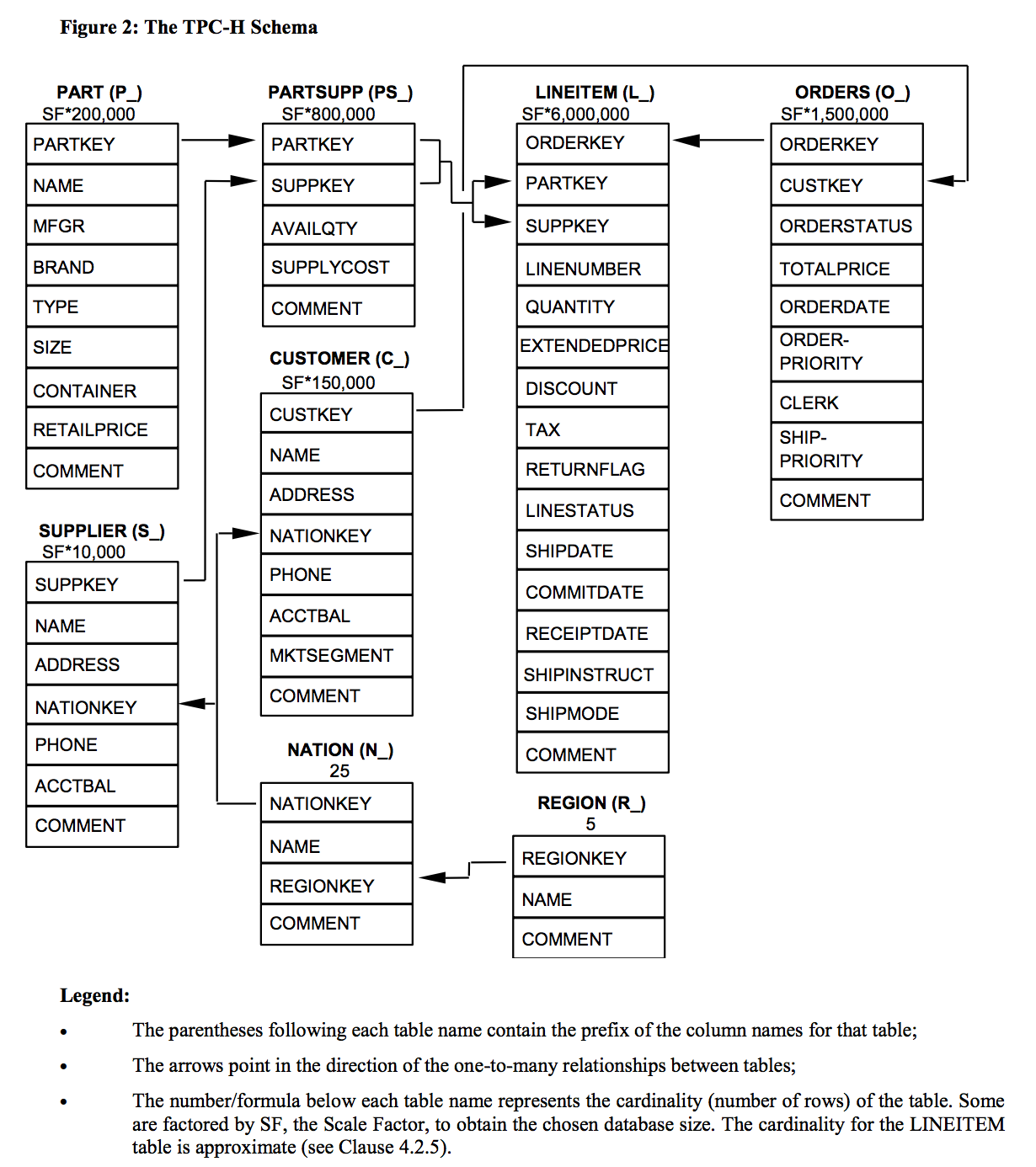
The exercises in this guide use the sample data provided with Snowflake trial accounts. This data is focused on fictitious commercial business data including supplier, customer, and orders information. For a full overview of the TPC-H schema, please visit Snowflake's documentation.
Before You Start
To complete this lab, please create free trial accounts with Snowflake and Coalesce by following the steps below. You have the option of setting up Git-based version control for your lab, but this is not required to perform the following exercises. Please note that none of your work will be committed to a repository unless you set Git up before developing.
We recommend using Google Chrome as your browser for the best experience.
Not following these steps will cause delays and reduce your time spent in the Coalesce environment.
Step 1: Create a Snowflake Trial Account
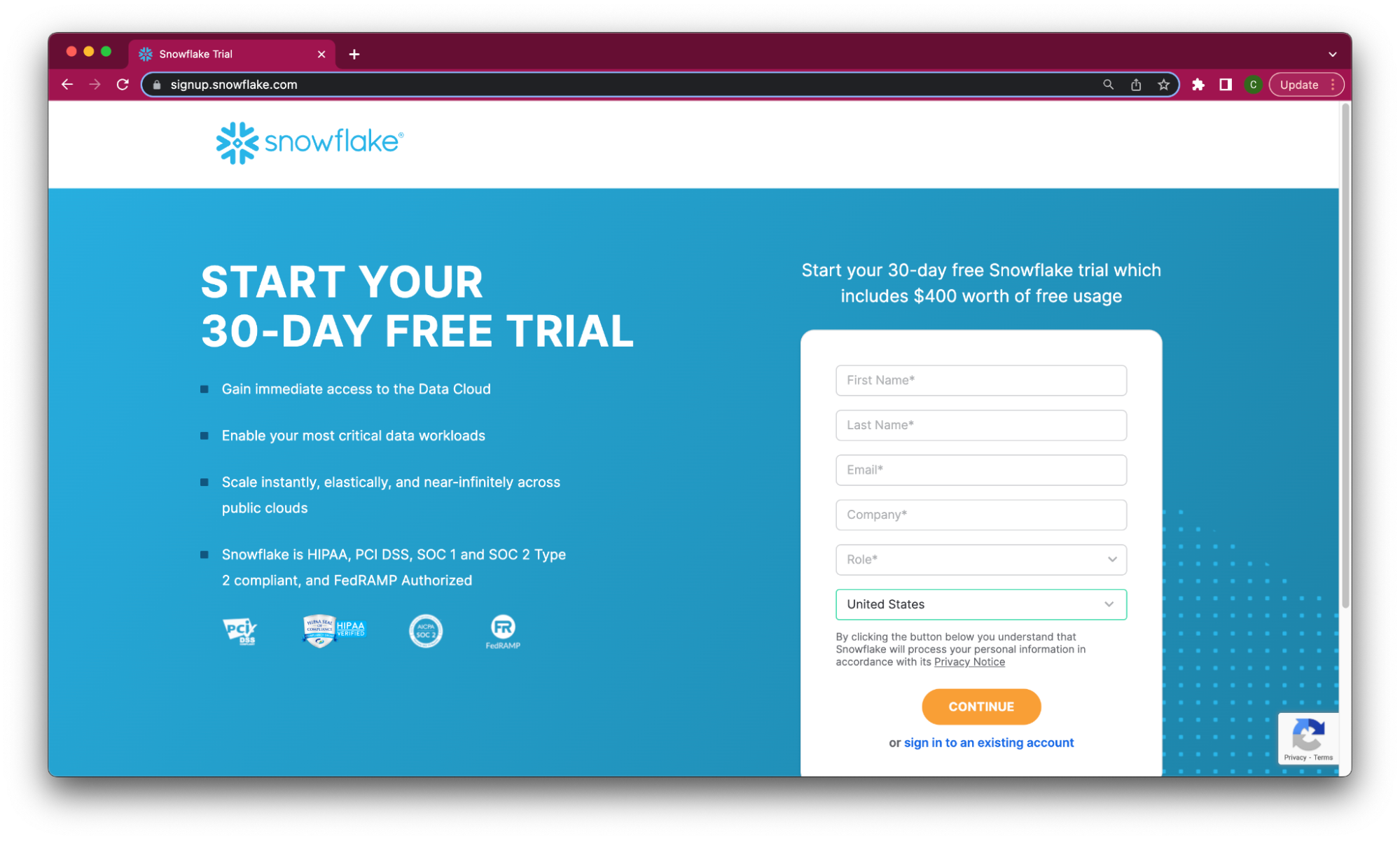
-
Fill out the Snowflake trial account form. Use an email address that is not associated with an existing Snowflake account.
-
After registering, you will receive an email from Snowflake with an activation link and URL for accessing your trial account. Finish setting up your account following the instructions in the email.
Step 2: Create a Coalesce Trial Account from Snowflake Marketplace
-
Sign in to Snowsight. Make sure you are using the ACCOUNTADMIN role (or a role with privileges to create a database, warehouse, user, and role) and that your Snowflake email address is verified.
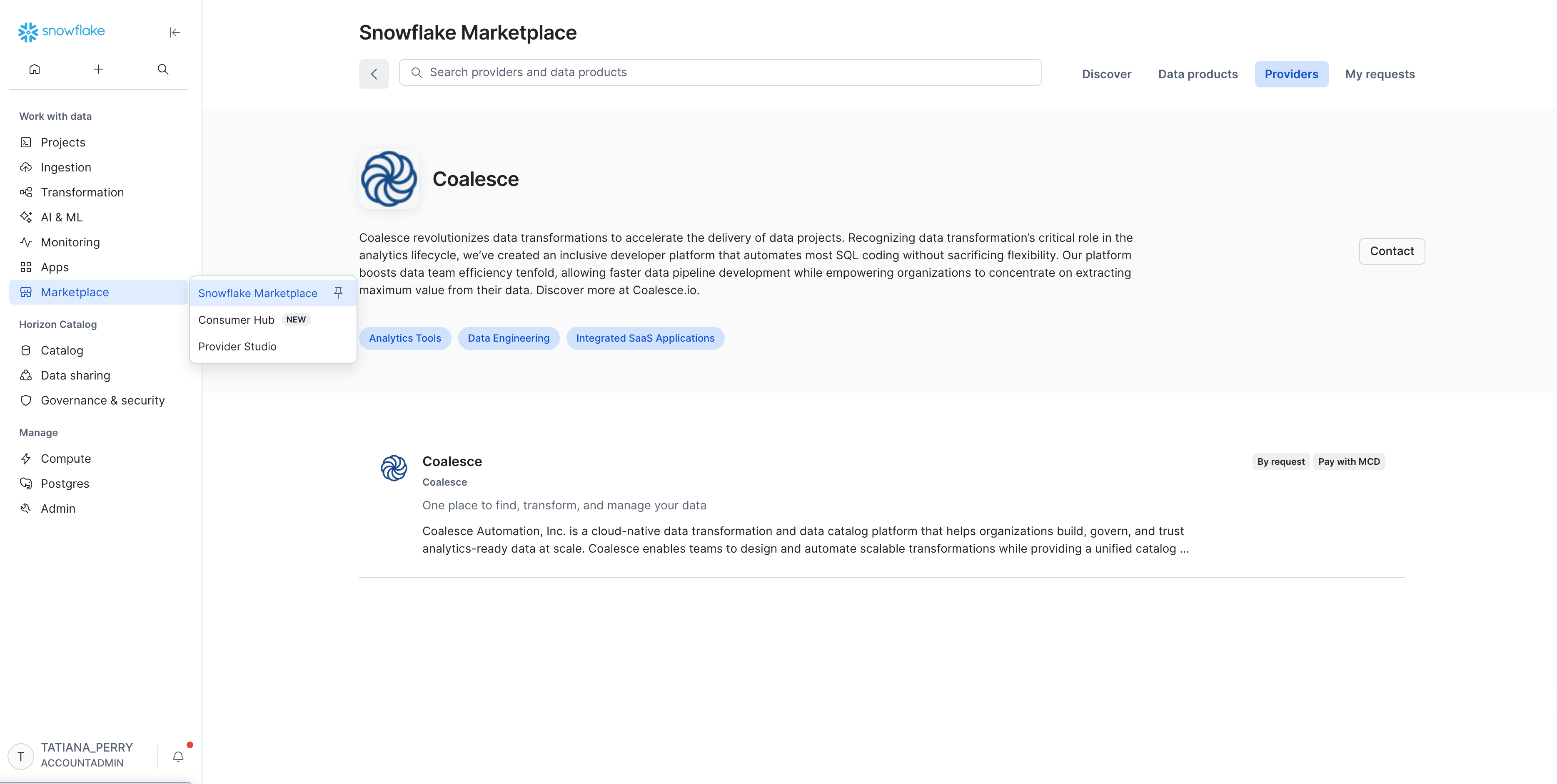
-
In the navigation menu, select Marketplace > Snowflake Marketplace and search for Coalesce.
-
Open the Coalesce listing and select Start free trial in the upper right. To see what the trial includes, review the Your free trial tab.
-
In the Connect to Coalesce dialog, review the information to be shared and the Snowflake objects that will be created, then select Connect to Coalesce.
-
You will be redirected to Coalesce to finish activating your trial account. Fill in your information to complete activation.
Congratulations. You’ve successfully created your Coalesce trial account.
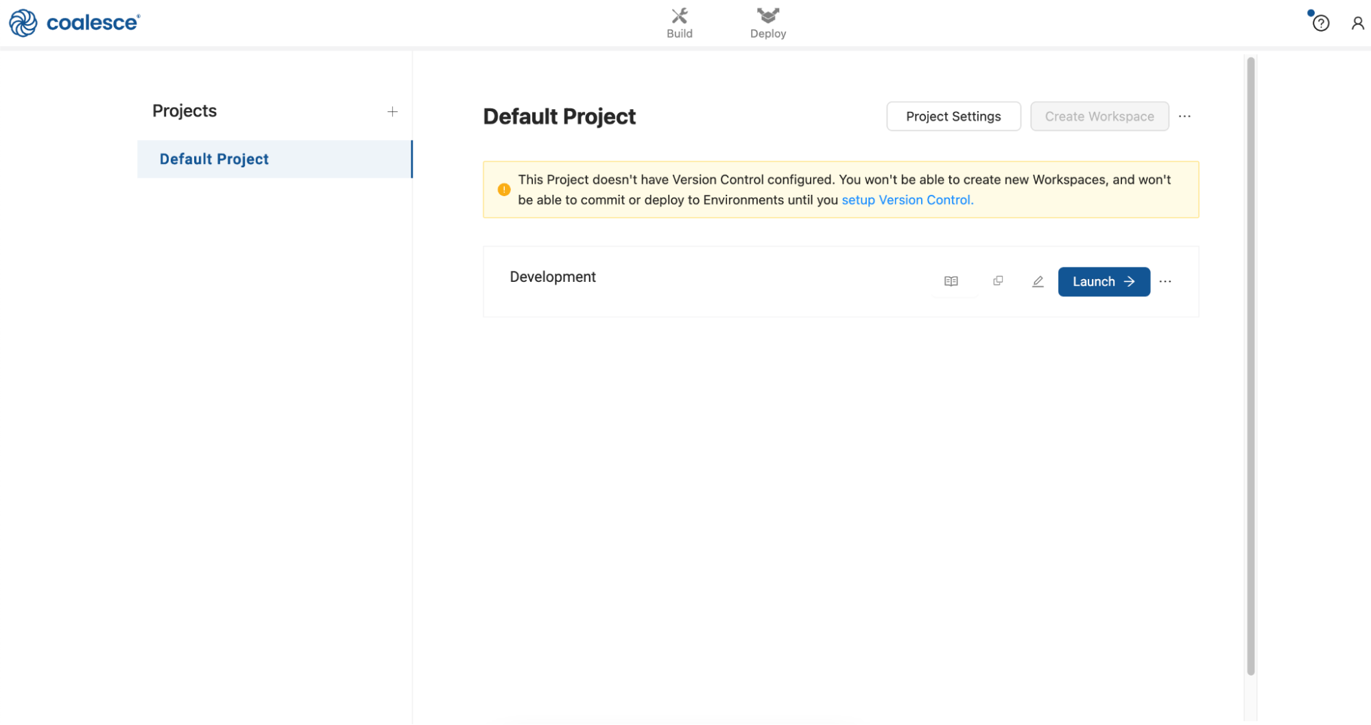
Once you’ve activated your Coalesce trial account and logged in, you will land in your Projects dashboard. Projects are a useful way of organizing your development work by a specific purpose or team goal, similar to how folders help you organize documents in Google Drive.
Your trial account includes a default Project to help you get started. Click on the Launch button next to your Development Workspace to get started.
Navigating the Coalesce User Interface
Screenshots (product images, sample code, environments) depict examples and results that may vary slightly from what you see when you complete the exercises.
This lab exercise does not include Git (version control). Please note that if you continue developing in your Coalesce account after this lab, none of your work will be saved or committed to a repository unless you set up before developing.
Let's get familiar with Coalesce by walking through the basic components of the user interface.
Upon launching your Development Workspace, you’ll be taken to the Build Interface of the Coalesce UI. The Build Interface is where you can create, modify, and publish nodes that will transform your data.
Nodes are visual representations of objects in Snowflake that can be arranged to create a Directed Acyclic Graph (DAG or Graph). A DAG is a conceptual representation of the nodes within your data pipeline and their relationships to and dependencies on each other.
-
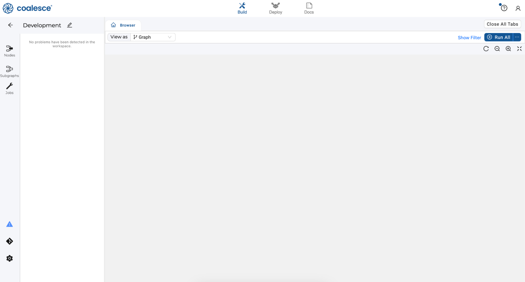
In the Browser tab of the Build interface, you can visualize your node graph using the Graph, Node Grid, and Column Grid views. In the upper right hand corner, there is a person-shaped icon where you can manage your account and user settings.

-
The Browser tab of the Build interface is where you’ll build your pipelines using nodes. You can visualize your graph of these nodes using the Graph, Node Grid, and Column Grid views. While this area is currently empty, we will build out nodes and our Graph in subsequent steps of this lab.
-
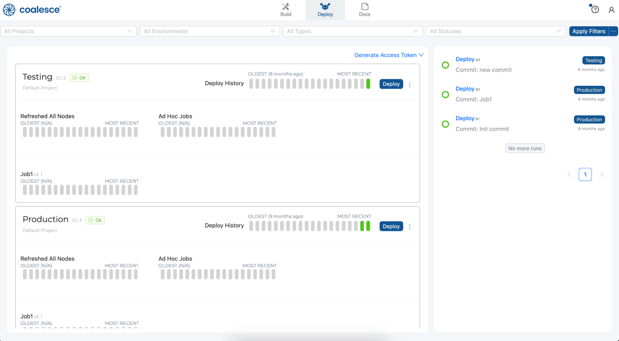
Next to the Build page is the Deploy page. This is where you will push your pipeline to other environments such as Testing or Production. Like the Browser tab, this area is currently empty but will populate as we will build out Nodes and our Graph in subsequent steps of this lab.
-
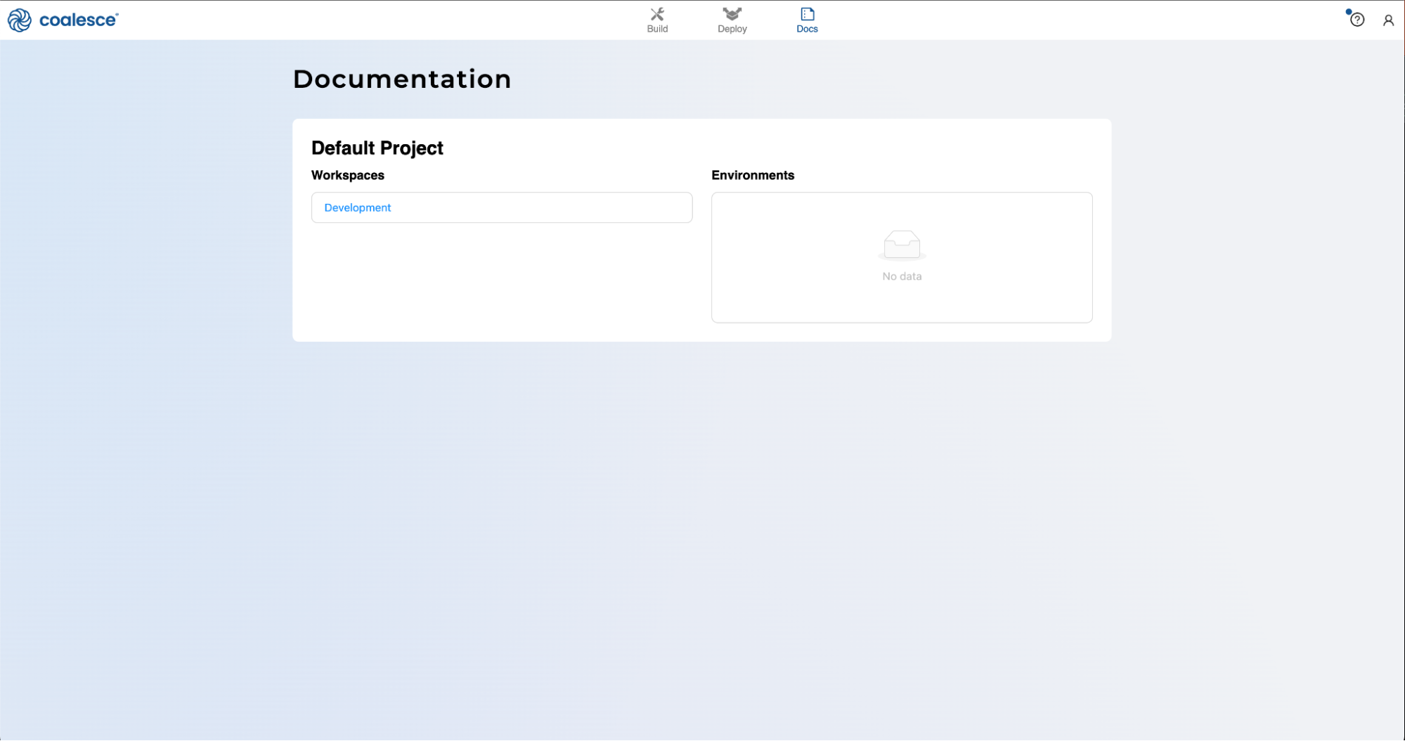
Next to the Deploy page is the Docs page. Documentation is an essential step in building a sustainable data architecture, but is sometimes put aside to focus on development work to meet deadlines. To help with this, Coalesce automatically generates and updates documentation as you work.
Adding Data Sources
Let’s start to build a Graph (DAG) by adding data in the form of Source nodes.
-
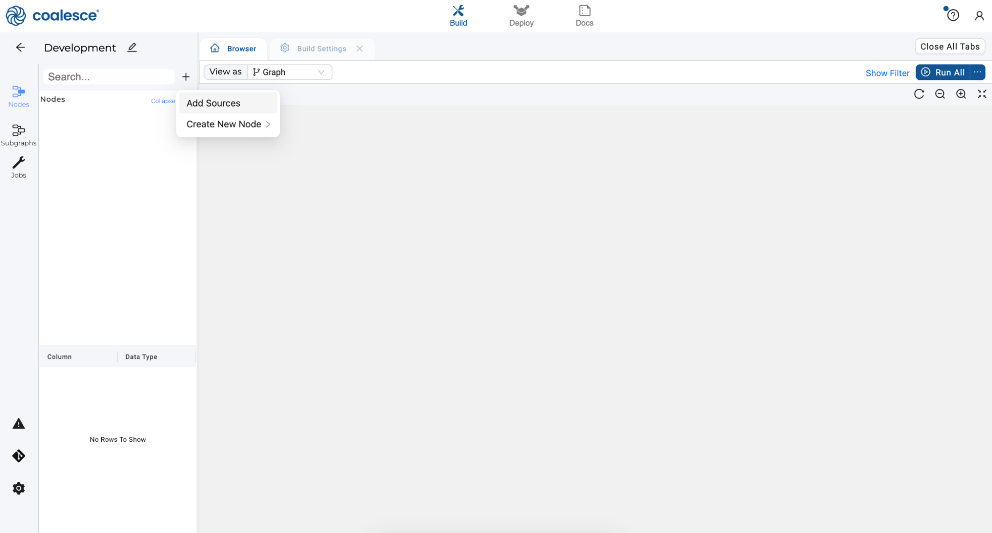
Start in the Build interface and click on Nodes in the left sidebar (if not already open). Click the + icon and select Add Sources.
-
Click to expand the tables within
COALESCE_SAMPLE DATABASE.TPCH_SF1and select all of the corresponding source tables underneath except forPARTSUPP(7 tables total). Click Add Sources on the bottom right to add the sources to your pipeline. You will use thePARTSUPPsource later on in this lab.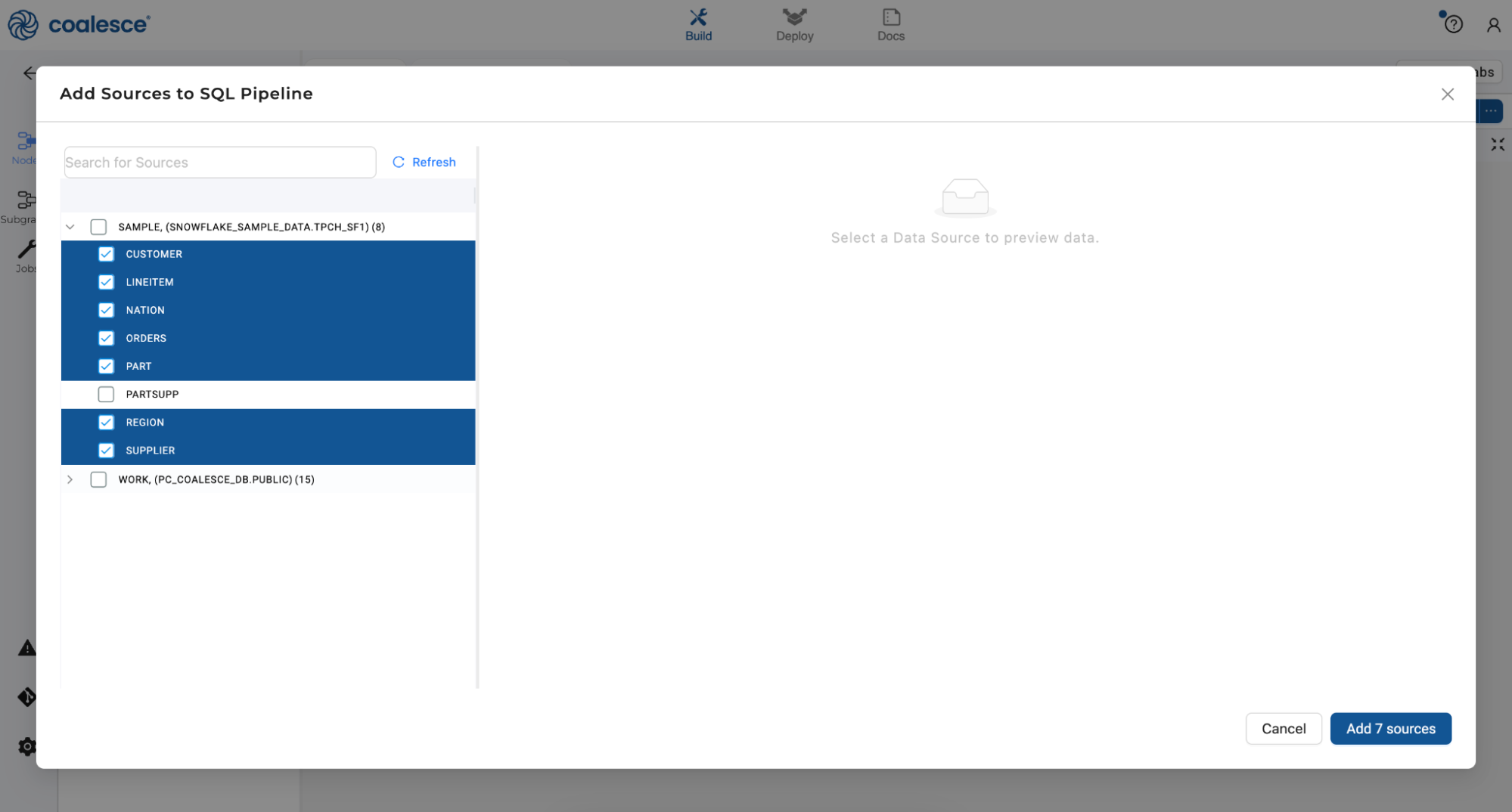
-
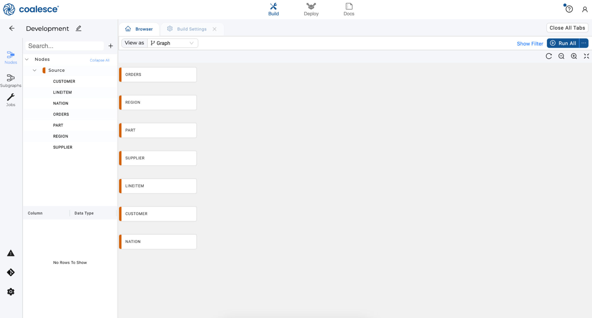
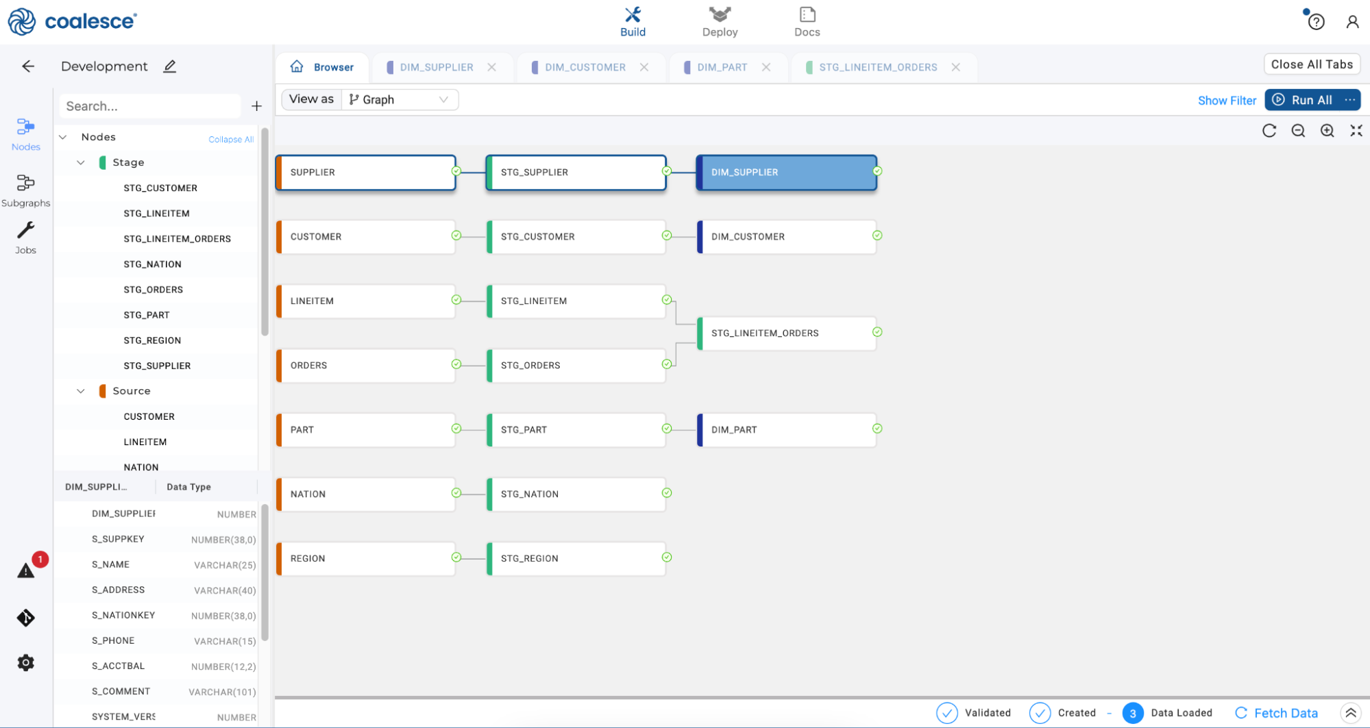
You'll now see your graph populated with your Source nodes. Note that they are designated in red. Each node type in Coalesce has its own color associated with it, which helps with visual organization when viewing a Graph.
Creating Stage Nodes
Now that you’ve added your Source nodes, let’s prepare the data by adding business logic with Stage nodes. Stage nodes represent staging tables within Snowflake where transformations can be previewed and performed.
Let's start by adding a standardized "stage layer" for all sources.
-
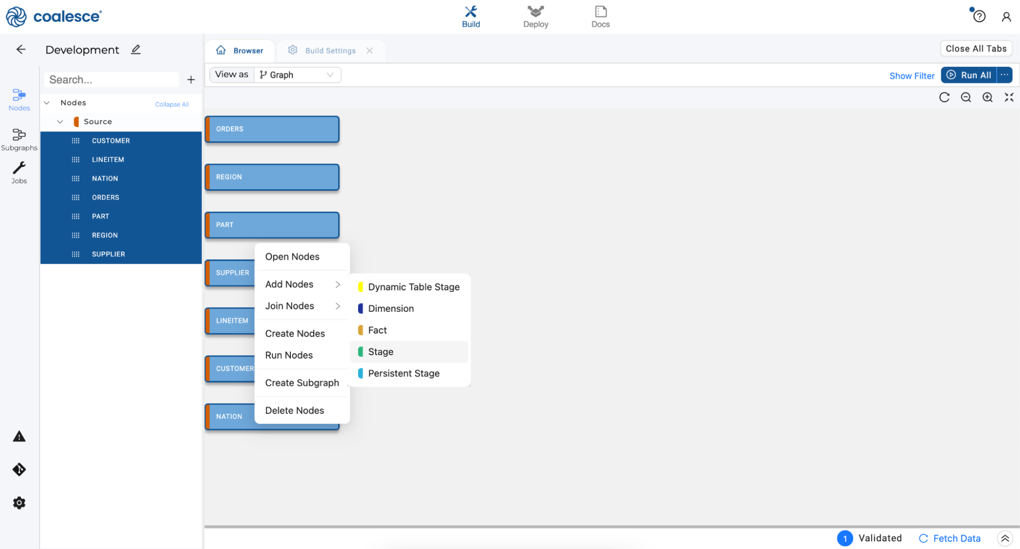
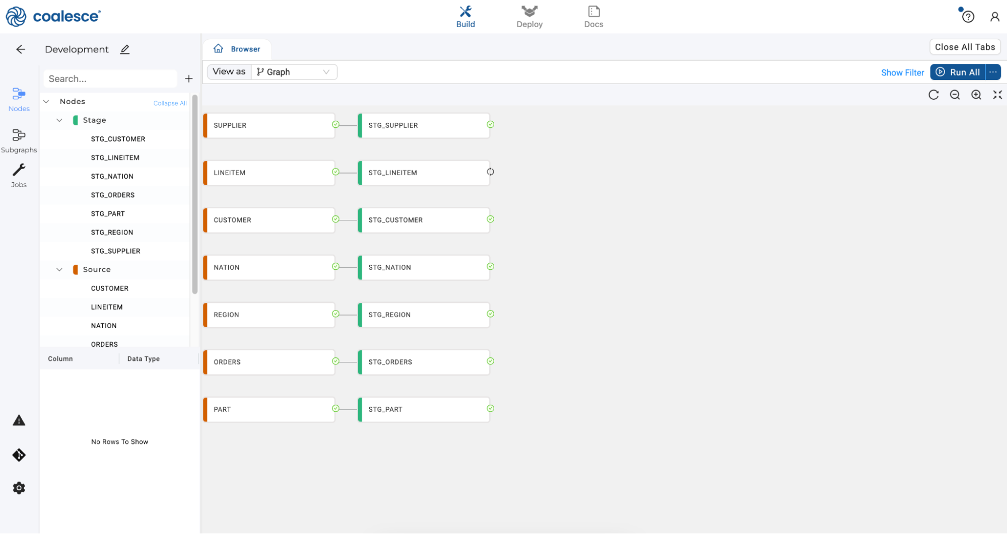
Press and hold the Shift key to multi-select all of your Source nodes. Then right click and select Add Node > Stage from the drop down menu.

You will now see that all of your Source nodes have corresponding Stage tables associated with them.
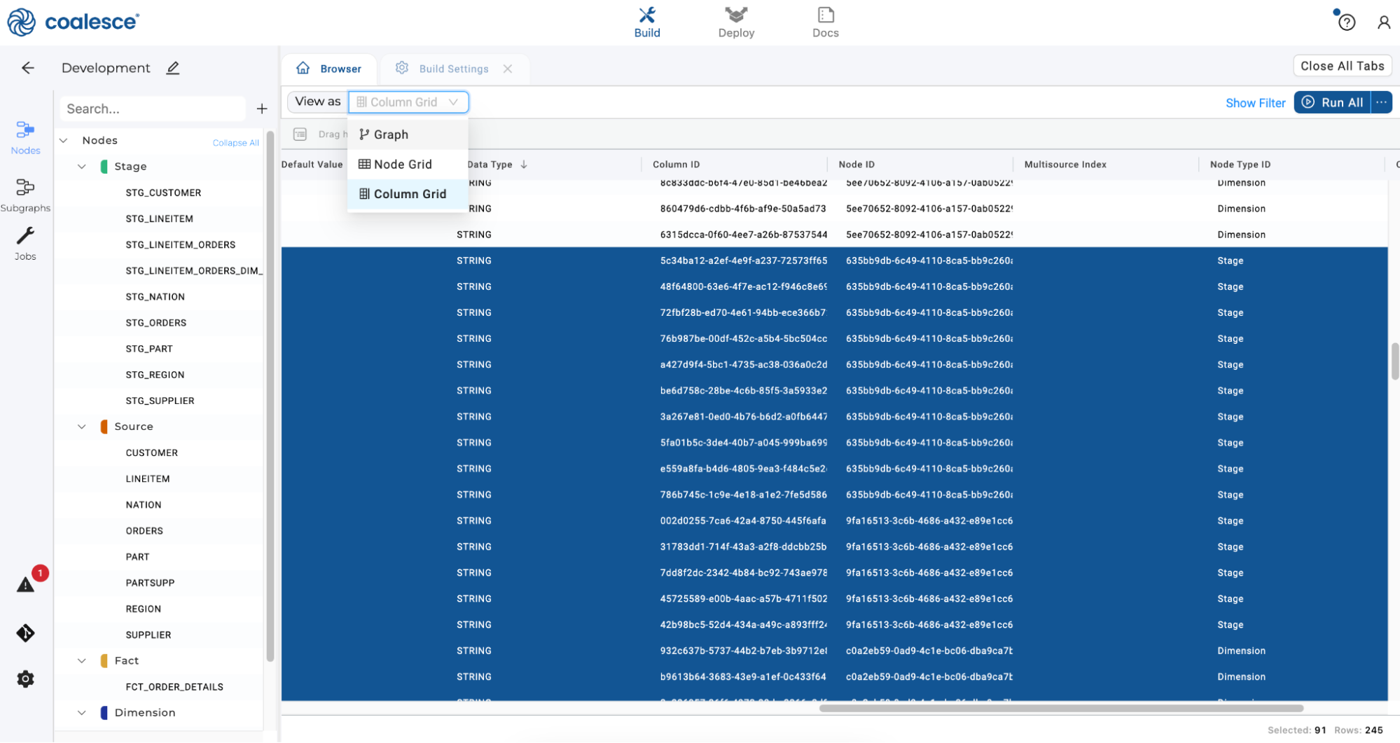
-
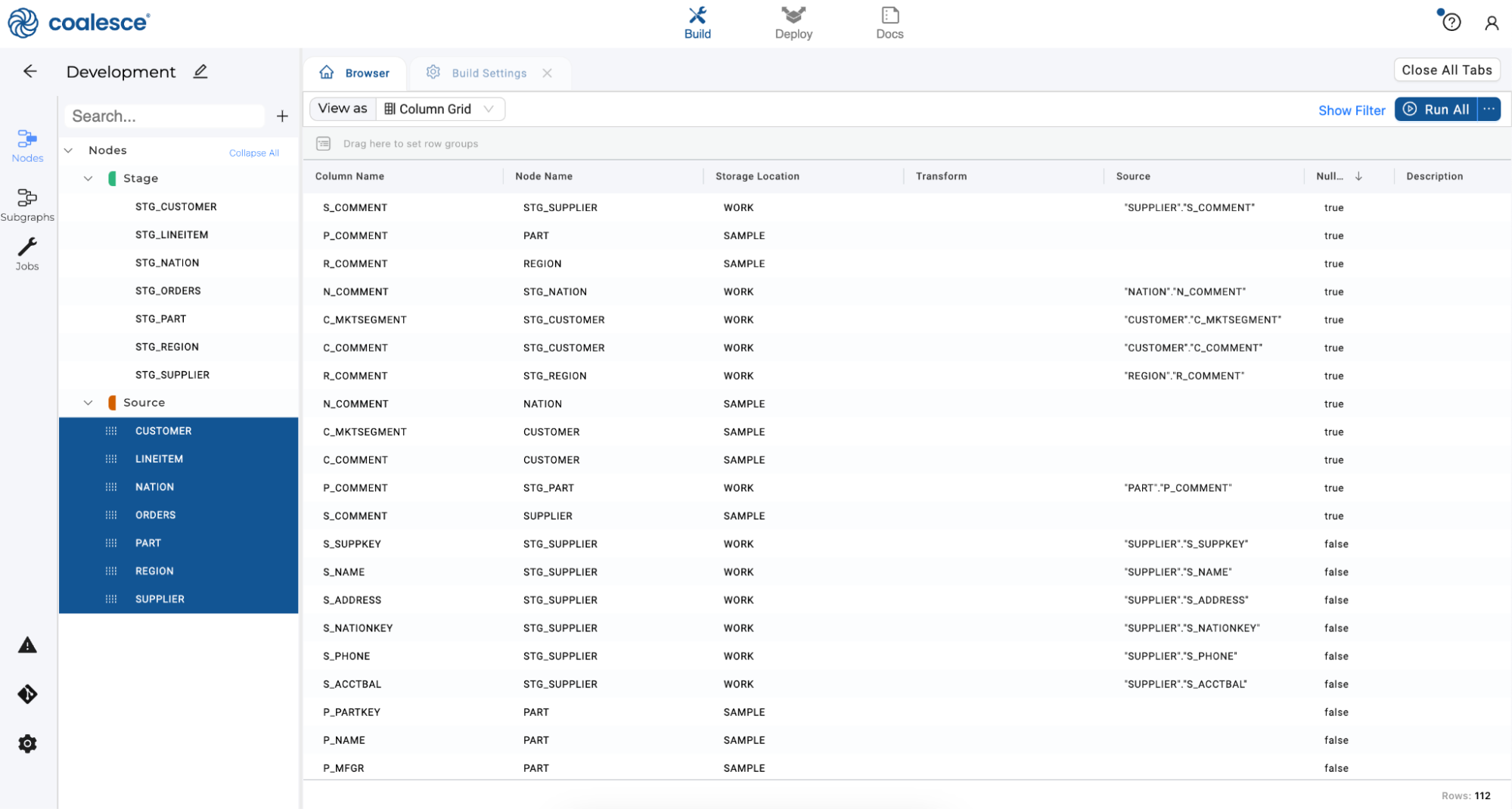
Now change the Graph to a Column Grid by using the top left dropdown menu:
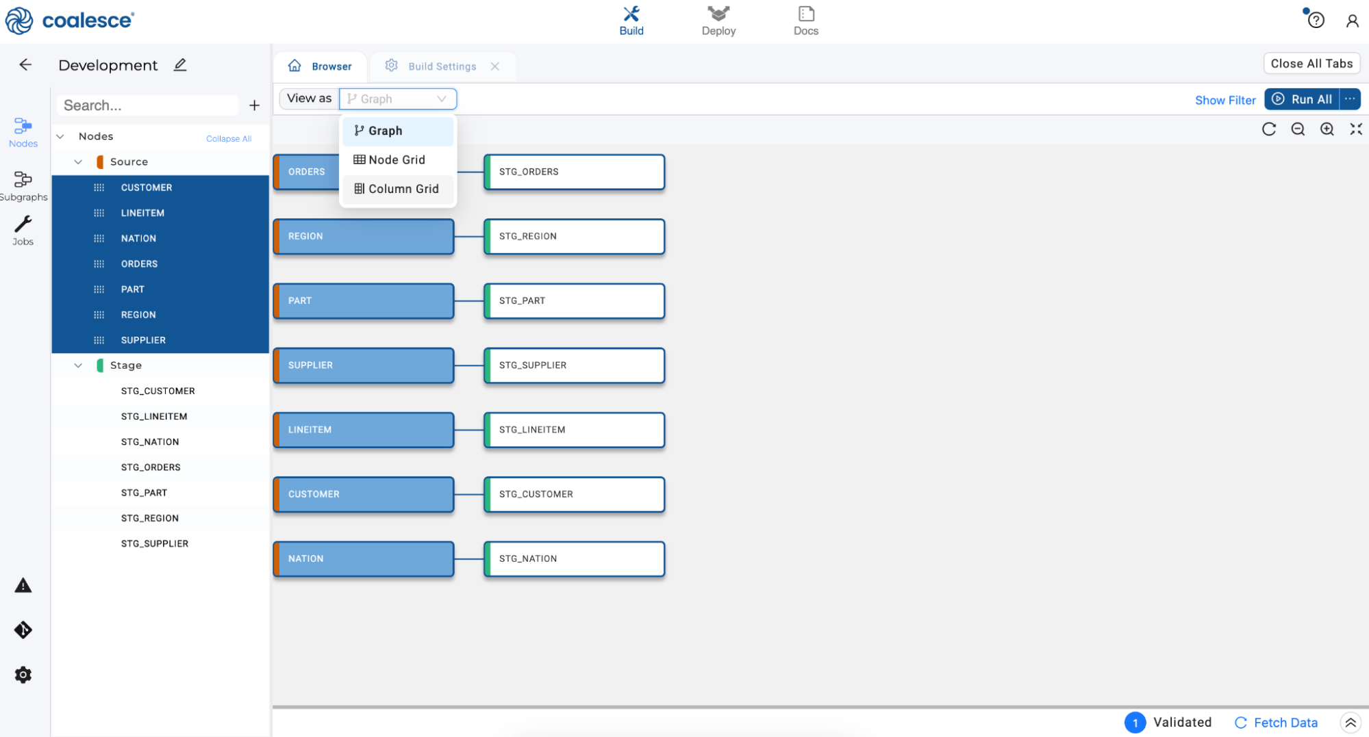
By using the Column Grid view, you can search and group by different column headers.
-
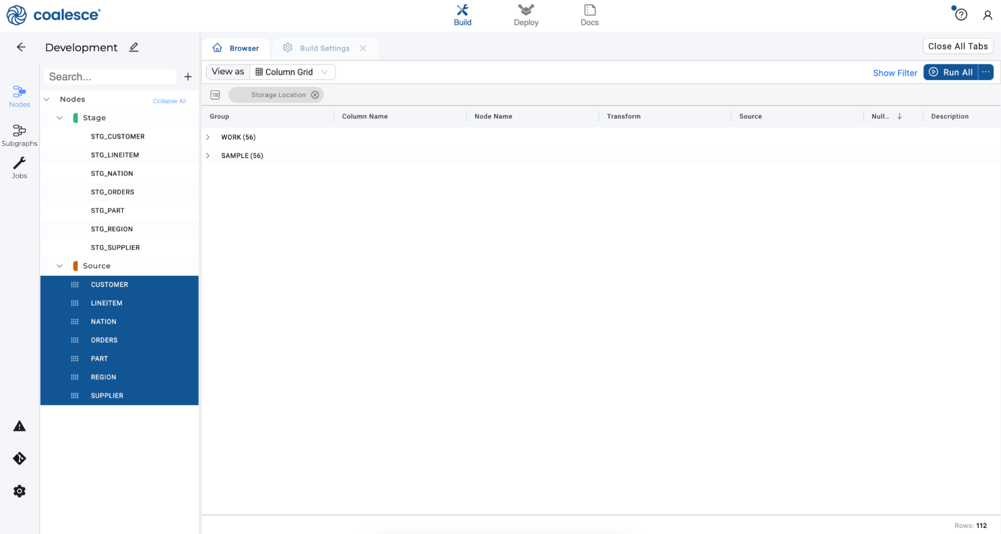
Click on the Storage Location header and drag it to the sorting bar below the View As dropdown menu. You have now grouped your rows by Storage Location.
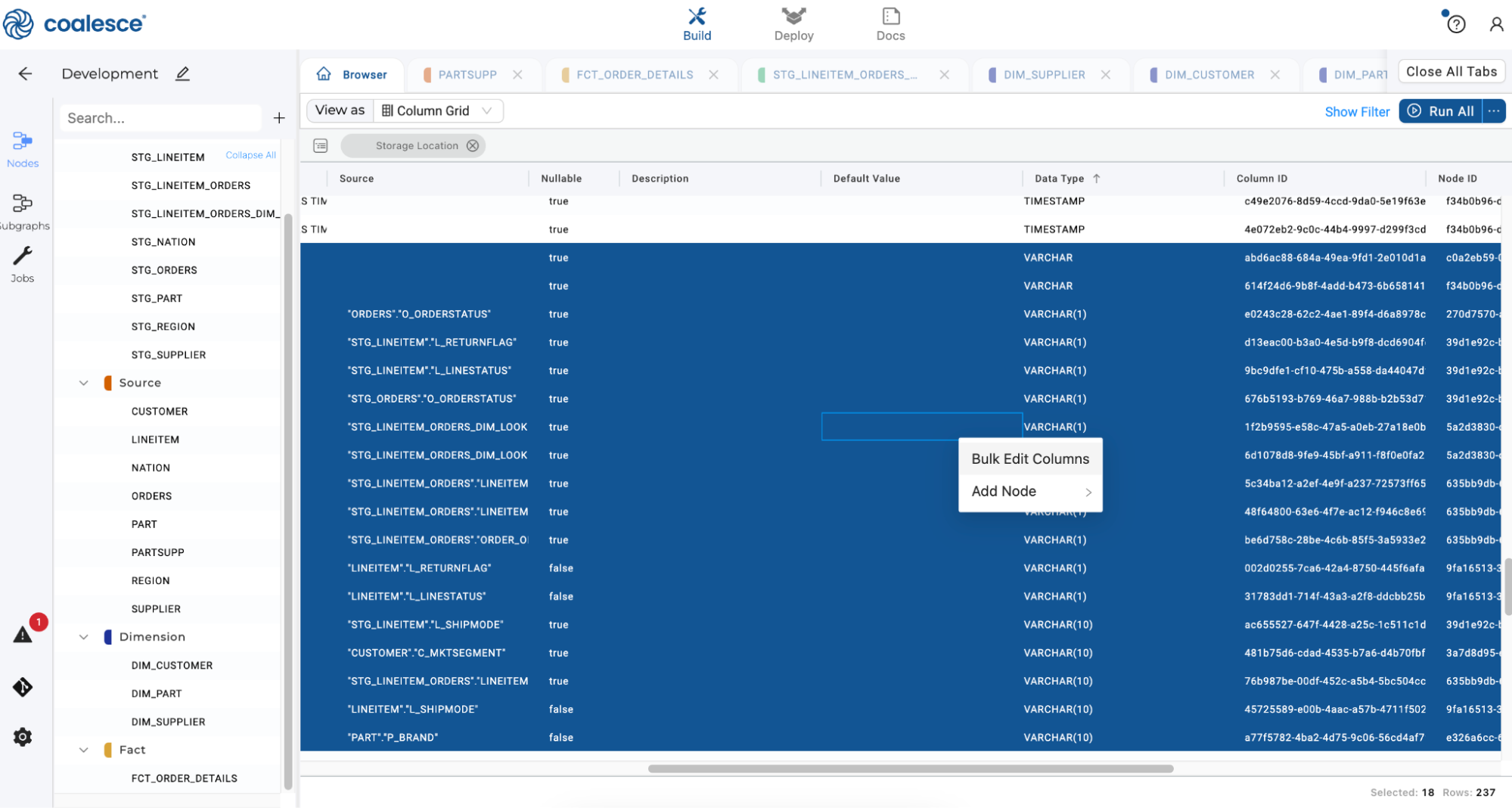
-
Expand all the columns from your
WORKlocation and select them. Then right click and select Bulk Edit Columns from the dropdown menu. Coalesce makes it quick and straightforward to apply transformations to your data by bulk editing columns.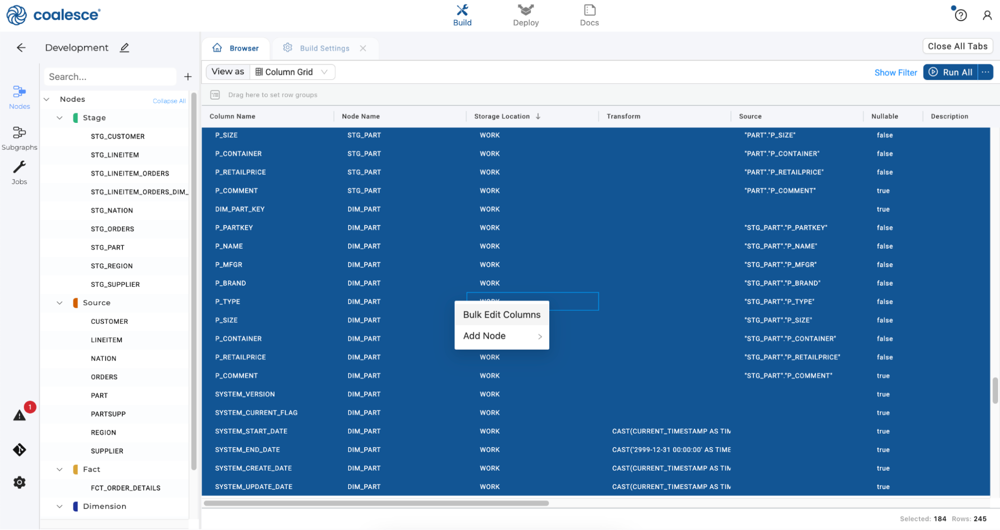
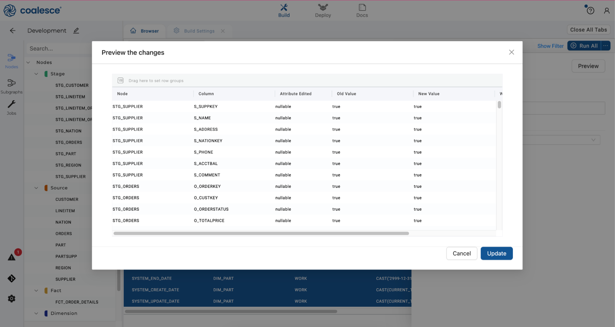
-
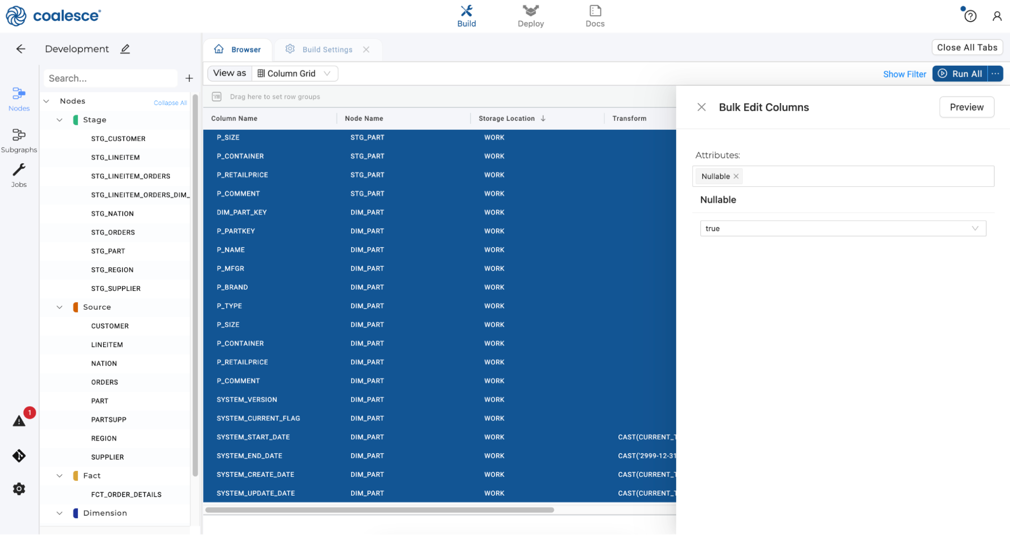
Select Nullable as an option and then True in the dropdown menu. This will make all columns in your WORK location nullable which will minimize any potential loading issues with the data.
-
Click the Preview button to preview your changes, and then click the Update button to apply them.
-
Repeat this step by scrolling to the right of your Column Grid and double clicking on the Data Type header so that VARCHAR values appear at the top of the grid. Press the Shift key and select all of the VARCHAR columns. Then right click and select Bulk Edit from the dropdown menu.
-
Select Data Type under Attributes and then type in STRING next to the Data Type field. By changing the data type to STRING as a bulk edit, we can minimize any potential issues with changes to our source data.

-
Click the Preview button once more and then press the Update button to make your changes. Then return to your Browser tab and change from Column Grid to Graph view with the dropdown menu.
-
Press the Create All button and then the Run All button to update your Graph.
Exploring the Node Editor
Now that we have a standard layer for performing basic transformations, let's add a more specific transformation by joining two of our Stage nodes. We’ll complete this in the Node Editor, which is used to edit the node object, the columns within it, and its relationship to other nodes
-
Press the Shift key and select the STG_LINEITEM and STG_ORDERS nodes. Once selected, right click and select Join Nodes > Stage to create a Stage node.
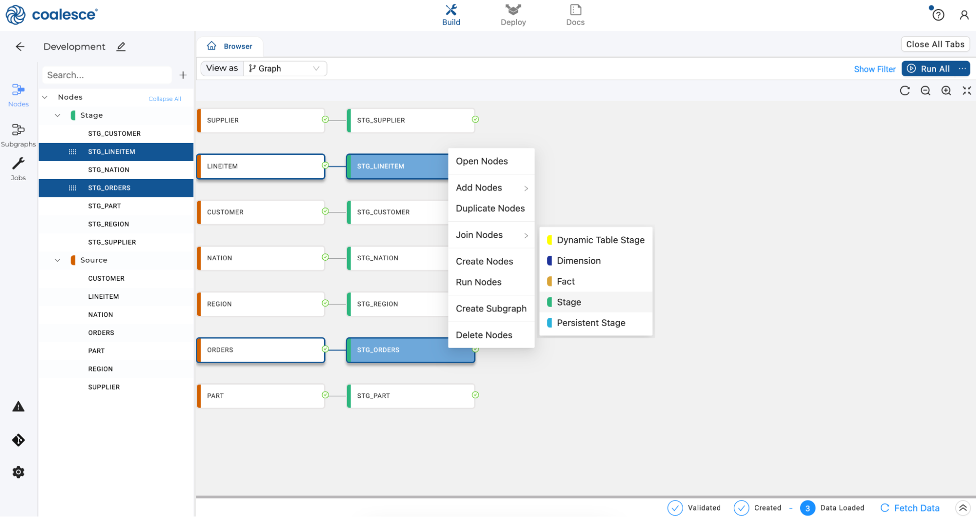
-
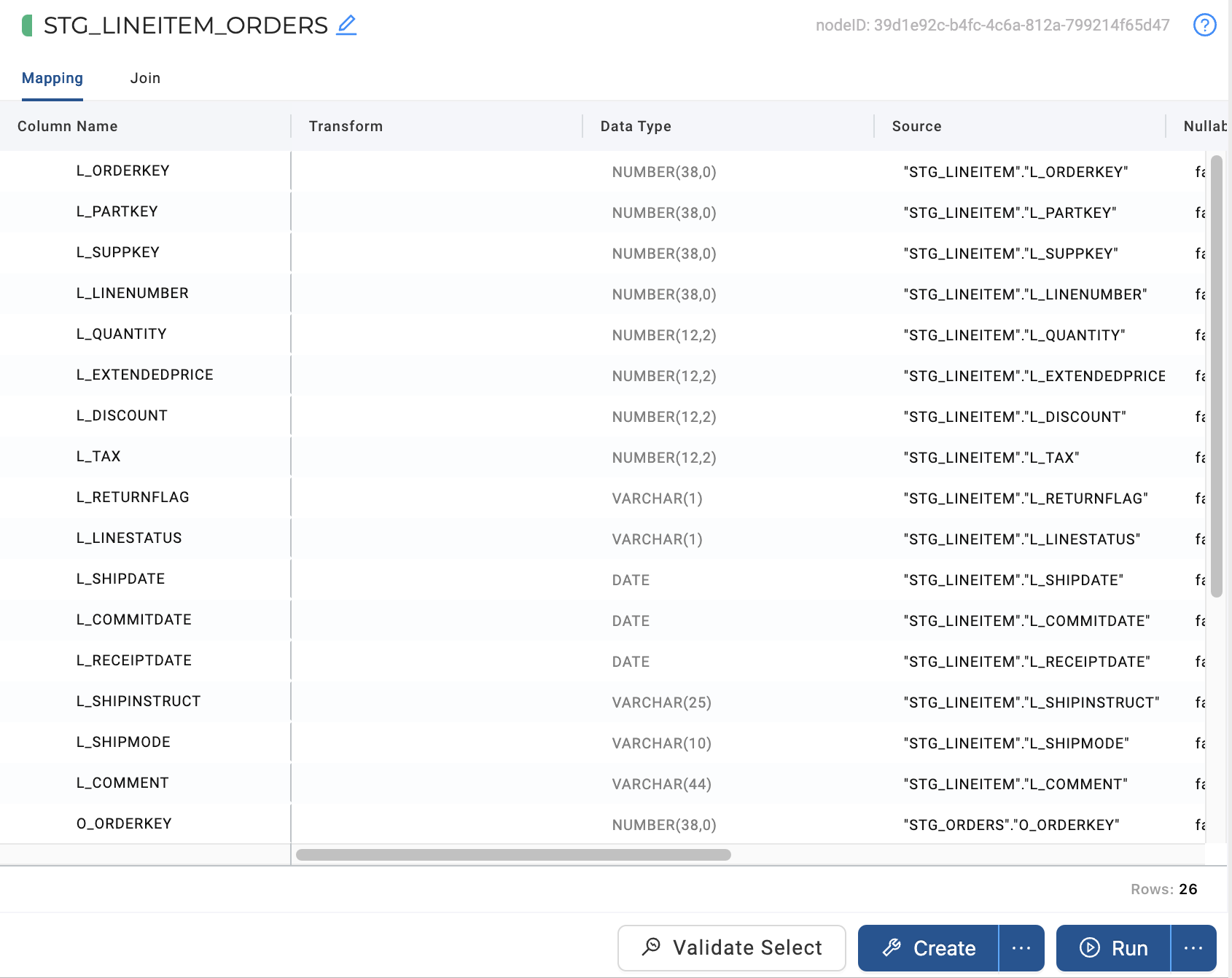
This action will cause a separate Node Editor tab to open up, which will appear next to your Browser tab. This is the Node Editor for the STG_LINEITEM_ORDERS node you just created. There are a few different components to this tab, the first section is the Mapping grid, where you can see the structure of your node along with column metadata like transformations, data types, and sources.
-
On the right hand side of the Node Editor is the Config section, where you can view and set configurations based on the type of node you’re using.
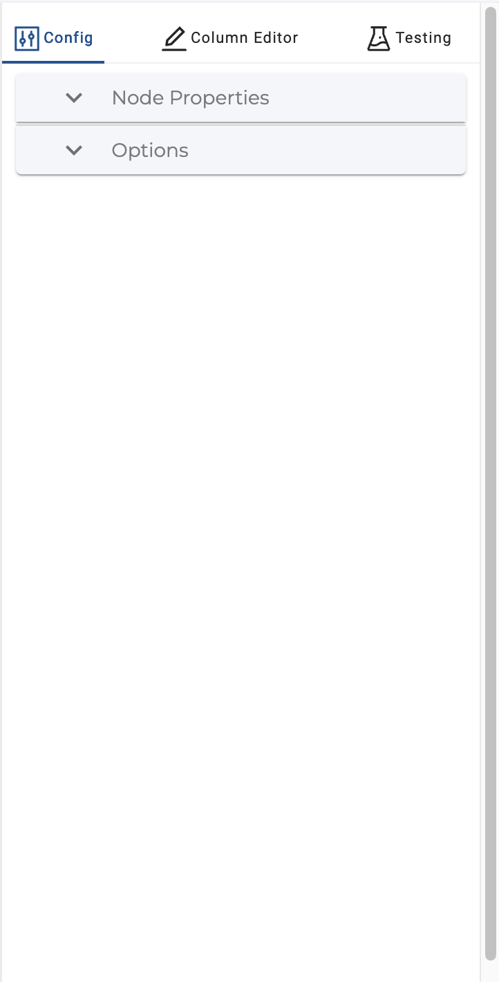
-
At the bottom of the Node Editor, press the arrow button to view the Data Preview pane.
Joining Nodes
Let’s now join your STG_ORDERS data with your STG_LINEITEM data.
-
Select the Join tab of your STG_LINEITEM_ORDERS node in the Node Editor. This is where you can define the logic to join data from multiple nodes, with the help of a generated Join statement.
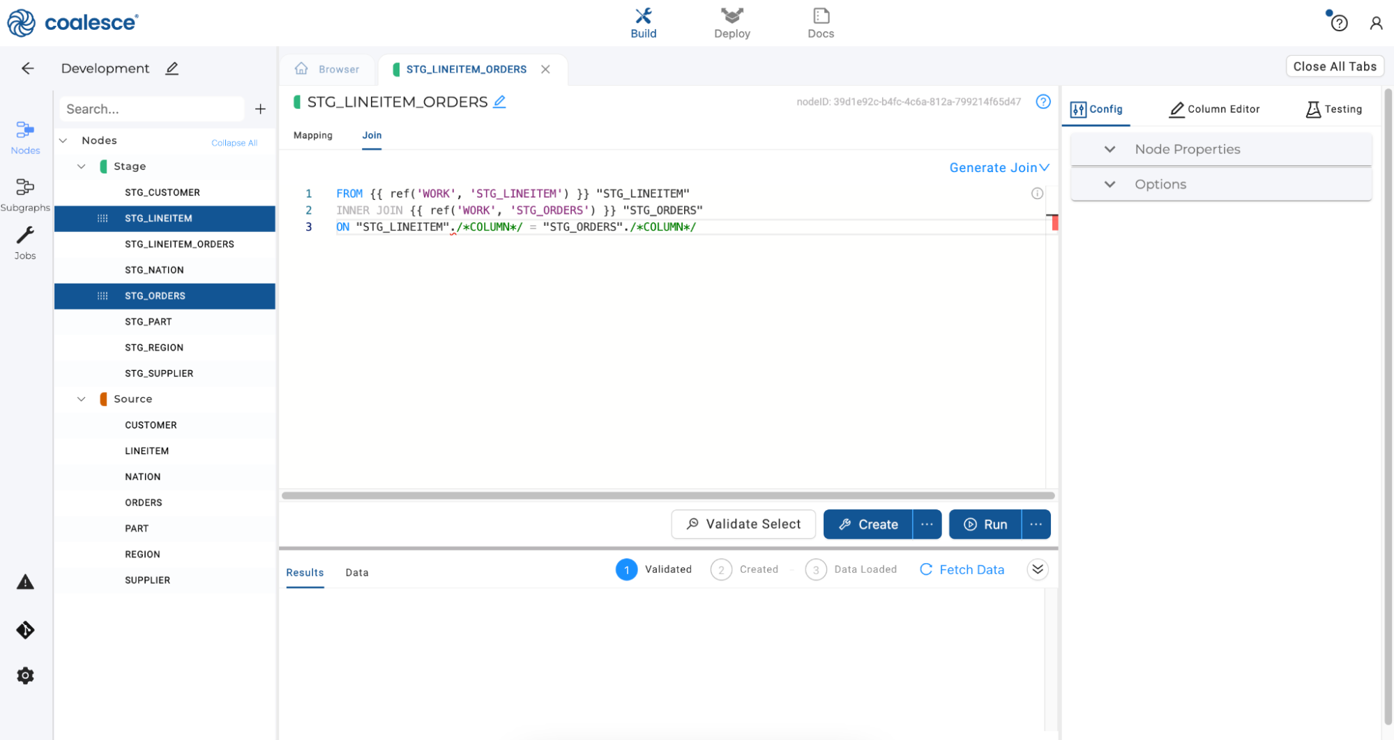
-
Add column relationships in the last line of the existing Join statement using the code below:
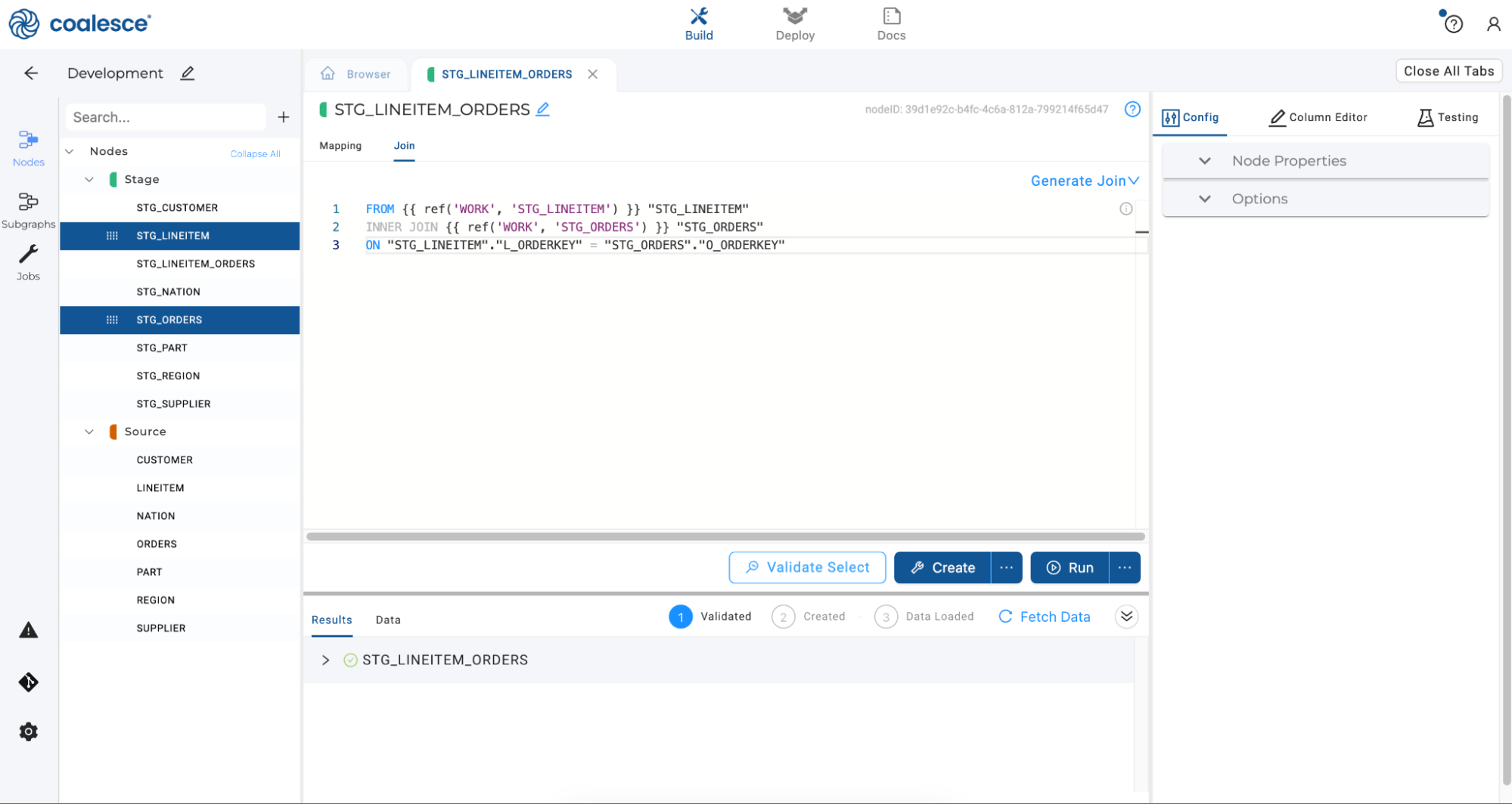
FROM {{ ref('WORK', 'STG_LINEITEM') }} "STG_LINEITEM"INNER JOIN {{ ref('WORK', 'STG_ORDERS') }} "STG_ORDERS"ON "STG_LINEITEM"."L_ORDERKEY" = "STG_ORDERS"."O_ORDERKEY" -
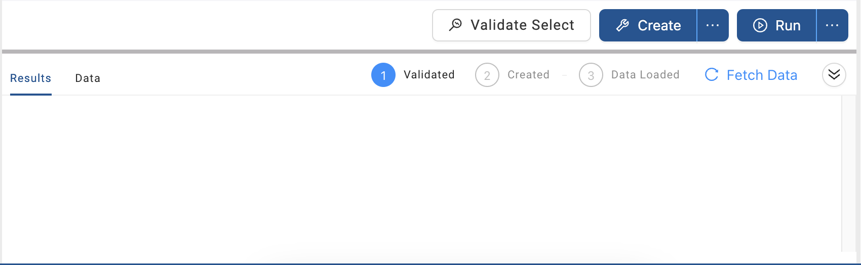
To check if your statement is syntactically correct, press the white Validate Select button in the lower half of the screen. The Results panel should show a green checkmark, confirming that the SQL is accepted. If not, you will see a database message indicating the error.
-
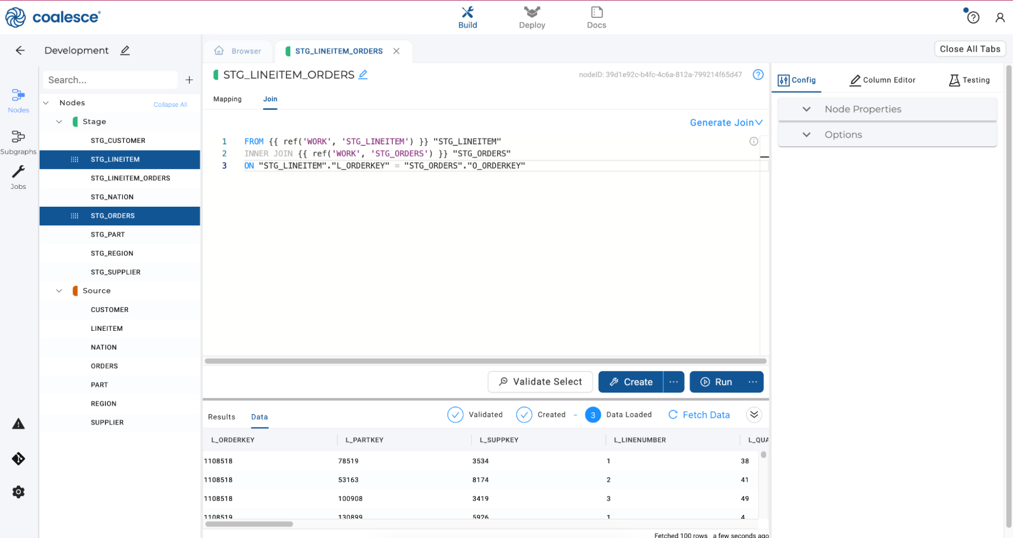
To create your Stage Node, click the Create button in the lower half of the screen. Then click the Run button to populate your STG_LINEITEM_ORDERS node and preview the contents of your node by clicking Fetch Data.
Applying Single Column Transformations
Let’s apply a single column transformation in your STG_LINEITEM_ORDERS node.
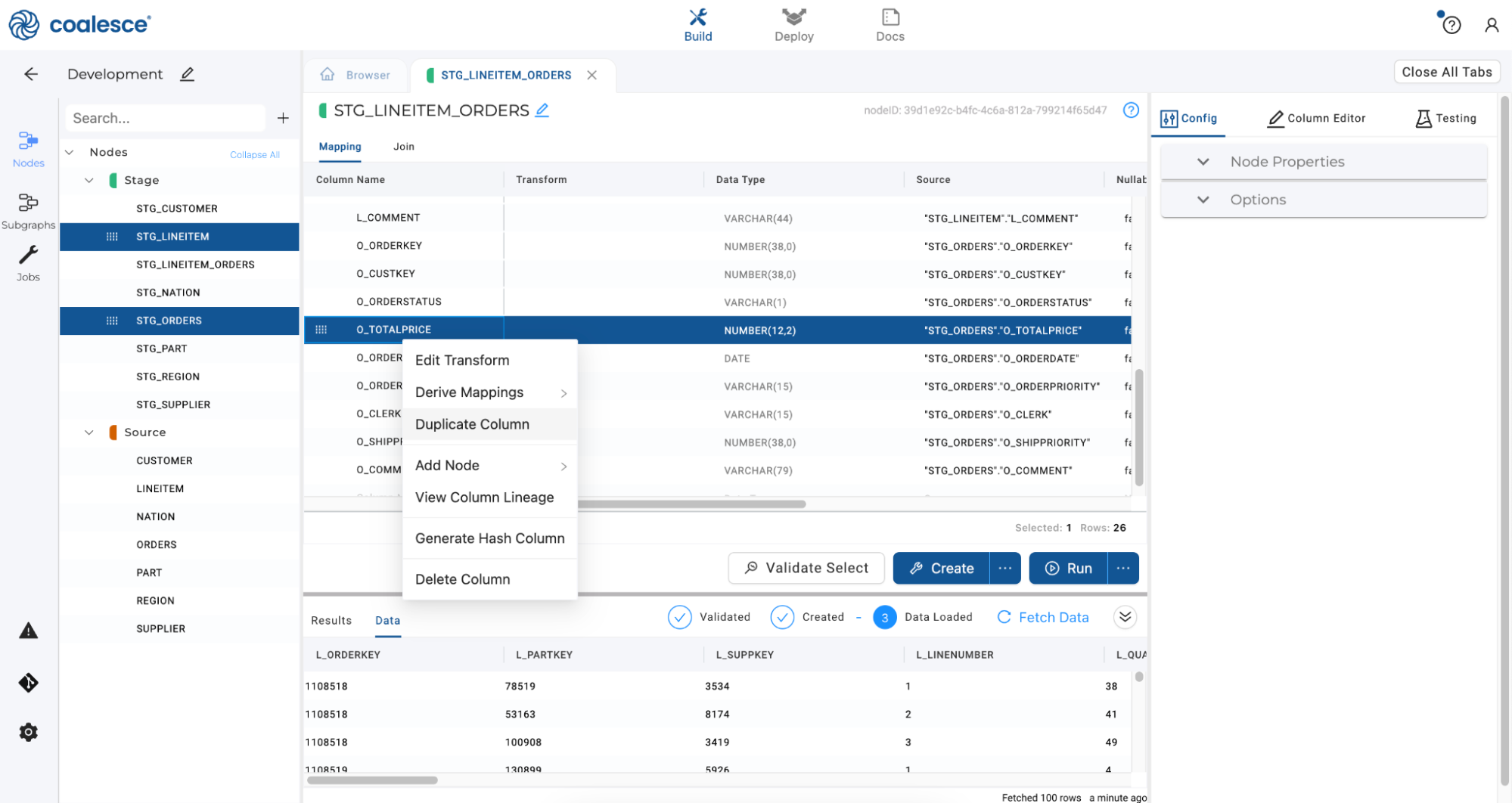
-
Click on Mapping to return to the Mapping Grid. Scroll down to the O_TOTALPRICE column and right click to duplicate the column.
-
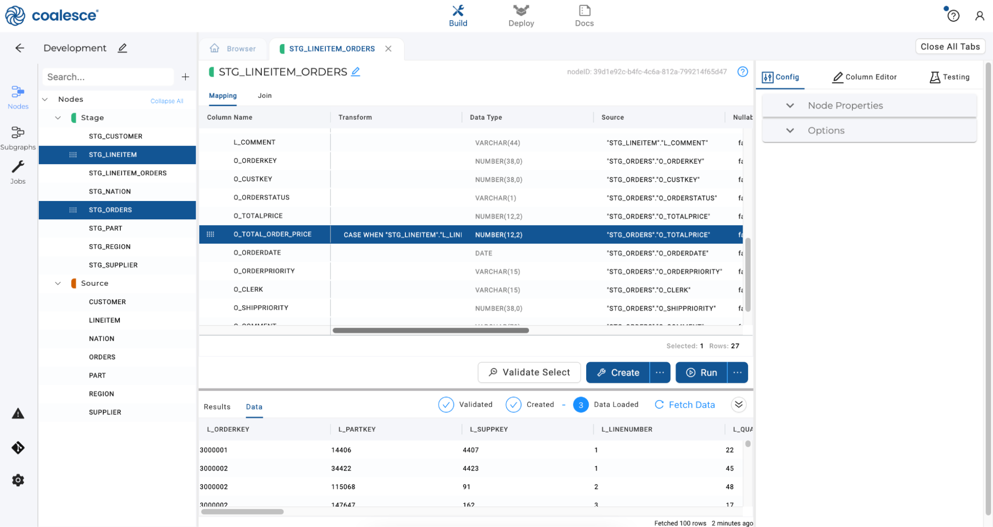
Double click on the duplicated column and rename it to
O_TOTAL_ORDER_PRICE. Then enter the transformation below in the Transform field to the right of the column name.CASE WHEN "STG_LINEITEM"."L_LINENUMBER" = 1 THEN {{SRC}} ELSE 0 ENDThe token
{{SRC}}serves as a shorthand for our source node, allowing us to perform the transformation faster without having to code individual source names by hand.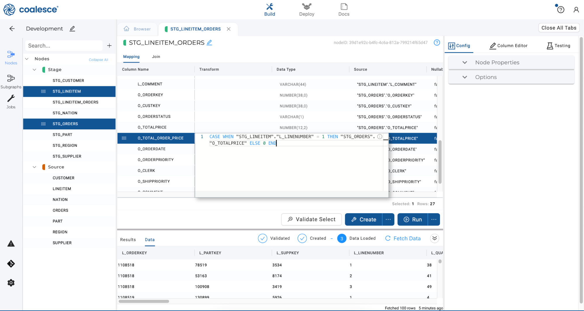
-
Click the Create and Run buttons once more to repopulate your node.
-
Click back to Mapping and scroll down in the Mapping grid to select the
O_ORDERPRIORITYcolumn. Rename the column asO_ORDERPRIORITY_NUMand enter the transformationSPLIT_PART("STG_ORDERS"."O_ORDERPRIORITY", '-', 1 )in the Transform field. This transformation formula takes the originalO_ORDERPRIORITYcolumn inSTG_ORDERS, splits its value at instances of '-', and returns the first portion of the split.Then right click on
O_ORDERPRIORITY_NUMcolumn and select Duplicate Column from the drop down menu.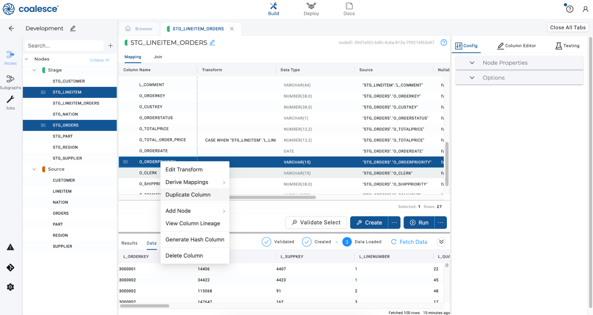
-
Rename the duplicate column as
O_ORDERPRIORITY_DESC.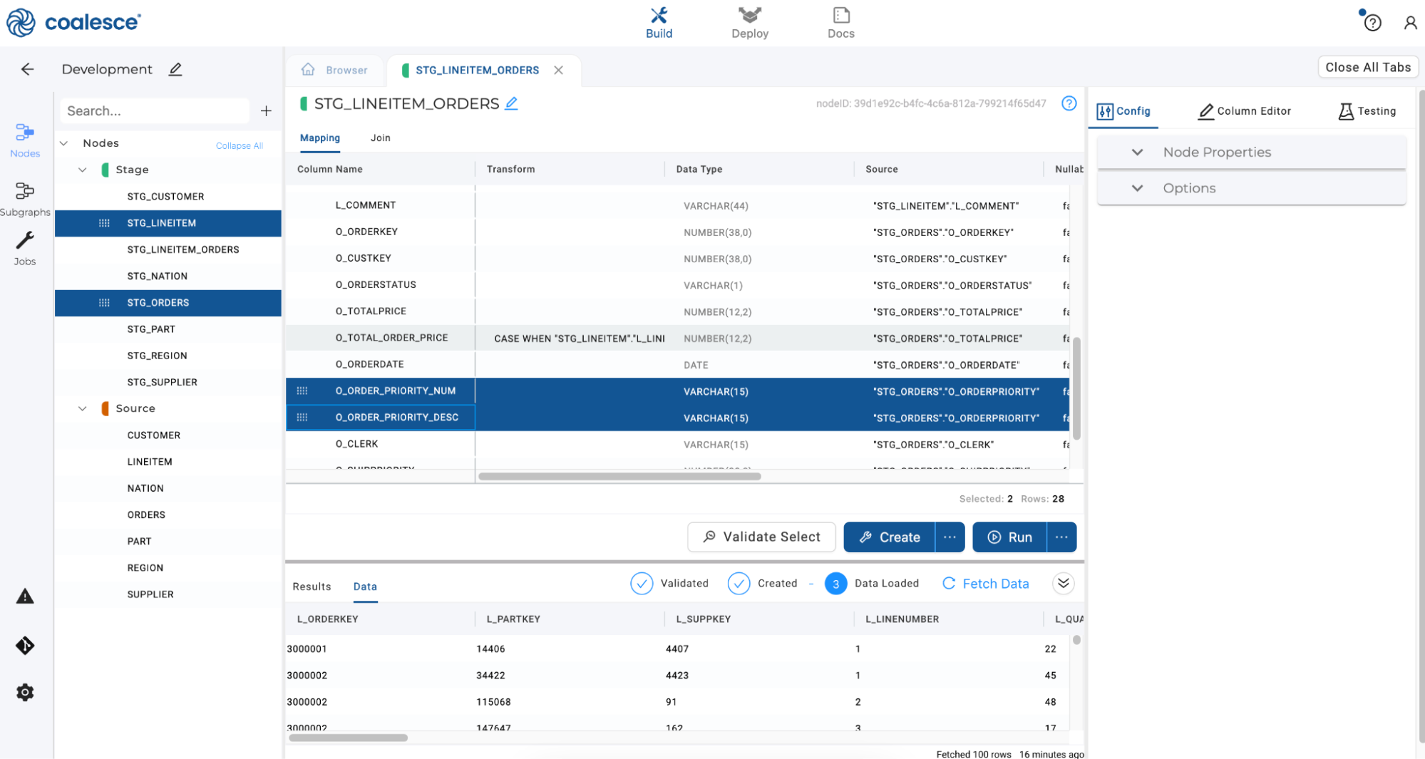
-
In the transform field for
O_ORDERPRIORITY_DESC, adjust the transformation to readSPLIT_PART("STG_ORDERS"."O_ORDERPRIORITY", '-', 2 ). Notice that this is the same transformation you entered previously, except this will now return the second portion of the split.Click the ellipsis on the Create button and select Validate Create to validate that your create statement will run. On confirmation, click Create and then click the Run button. Once the Run has completed, scroll to the right in the Data Preview pane to preview your new
O_ORDERPRIORITY_NUMandO_ORDERPRIORITY_DESCcolumns.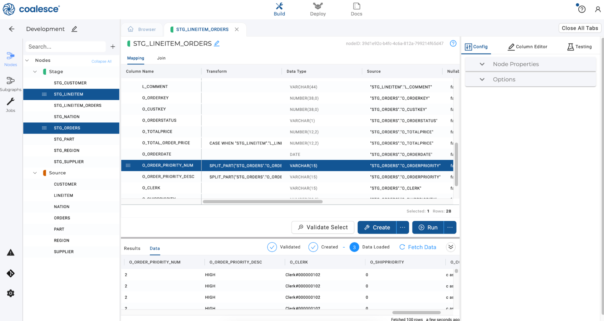
-
Now let’s apply another single column transformation by concatenating two different columns from different Stage nodes. Scroll to the bottom of the Mapping grid and double click on the gray column named Column Name.

-
Name this column
DAYS_TO_SHIPand press the Enter key to create a new column. Under Data Type, enterNUMBER.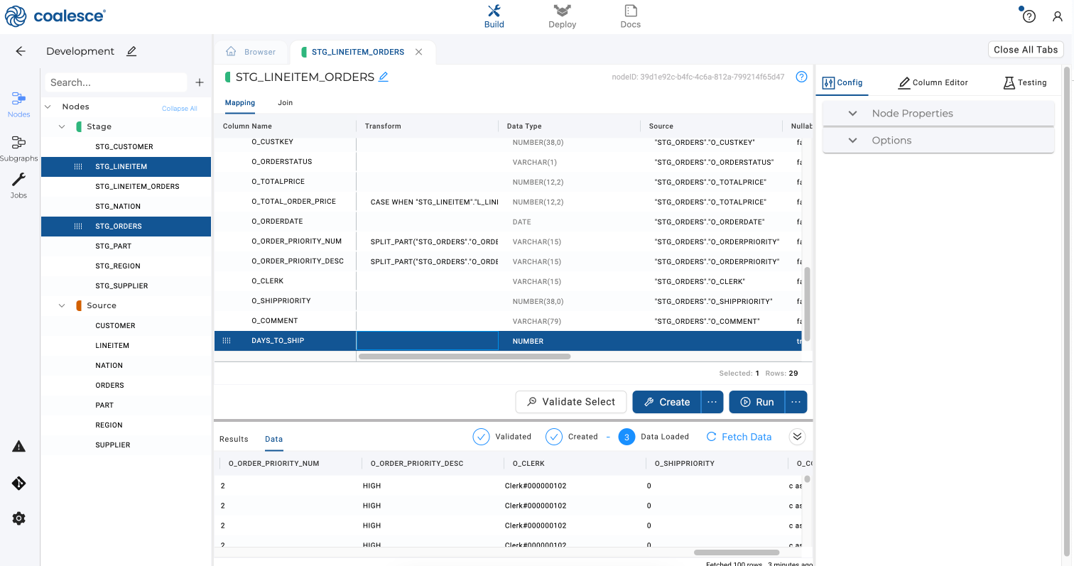
-
In the Transform field, enter the following transformation to calculate the difference between order dates and shipping dates listed in the
STG_ORDERSandSTG_LINEITEMnodes.DATEDIFF('DAY',"STG_ORDERS"."O_ORDERDATE","STG_LINEITEM"."L_SHIPDATE")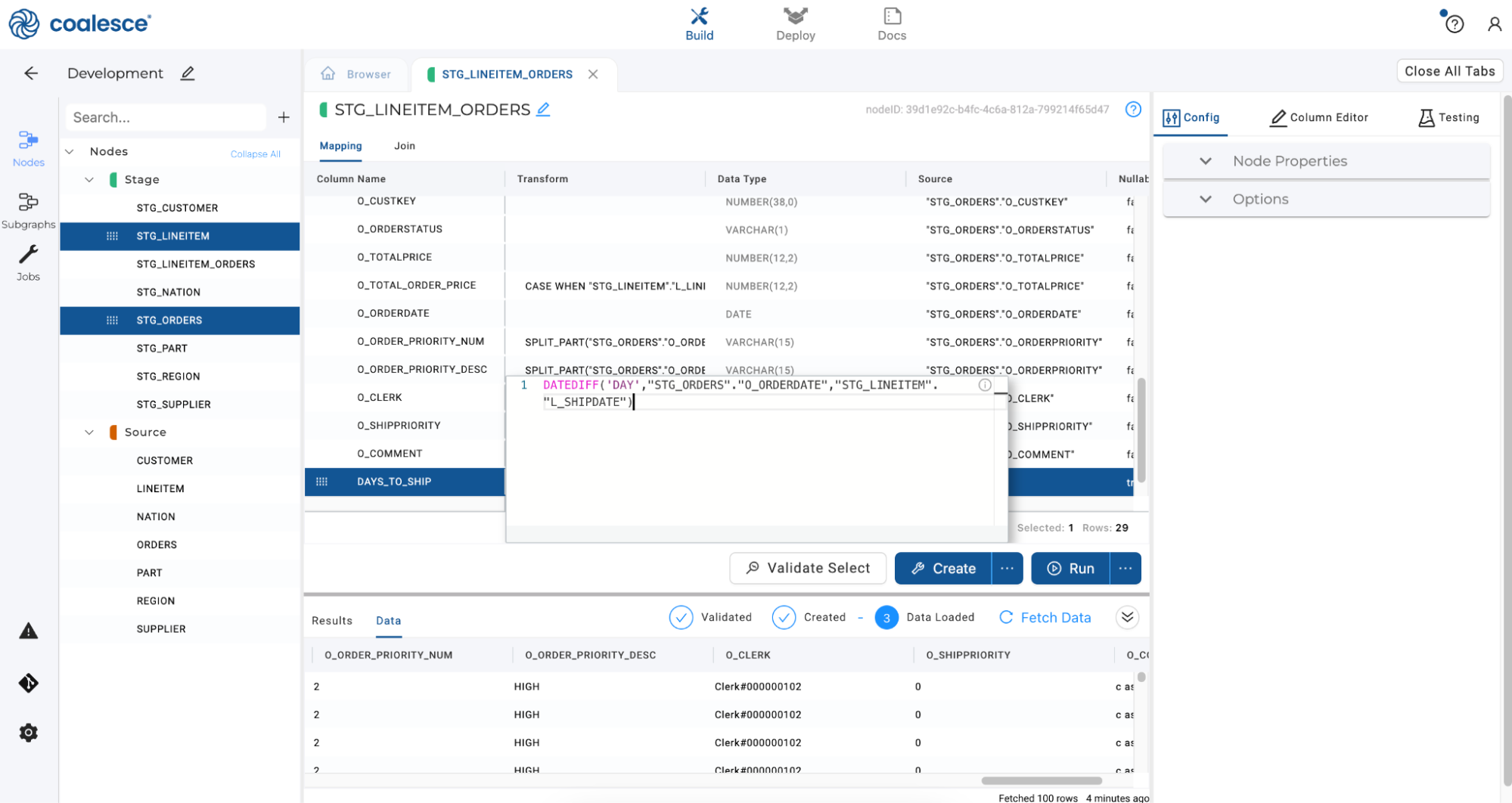
-
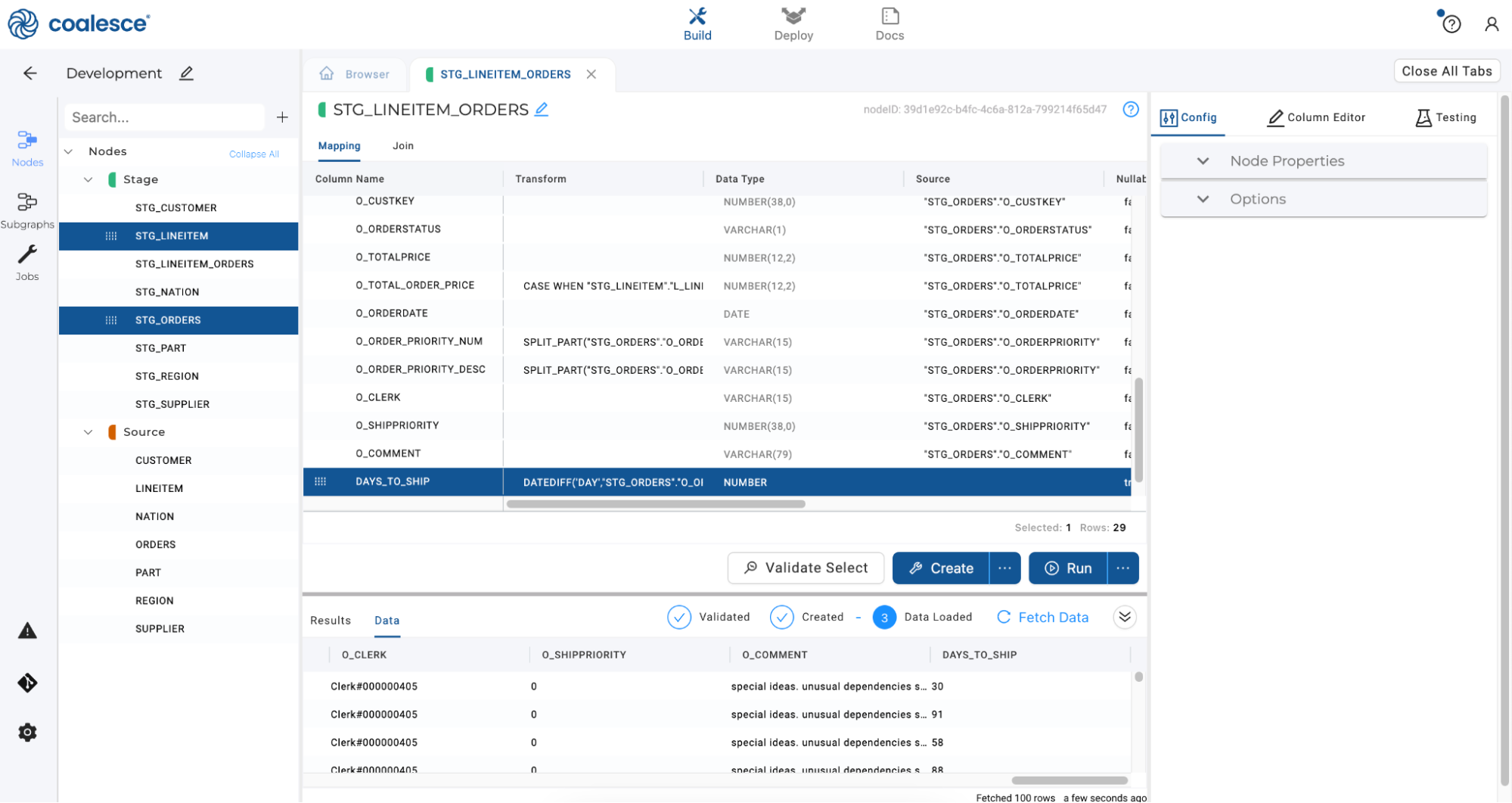
Click the Create and Run buttons to execute the statements. Once the Run has completed, scroll to the right in the Data Preview pane to view your newly created
DAYS_TO_SHIPcolumn.
Creating Dimension Nodes
Now let’s experiment with creating Dimension nodes. These nodes are generally descriptive in nature and can be used to track particular aspects of data over time (such as time or location). Coalesce currently supports Type 1 and Type 2 slowly changing dimensions, which we will explore in this section.
-
In your
STG_LINEITEM_ORDERSnode, navigate to the Mapping grid. Select theO_CUSTKEYcolumn and drag it to the top of the Mapping grid. Repeat this motion by dragging theL_SUPPKEYandL_PARTKEYcolumns to the top of the Mapping grid.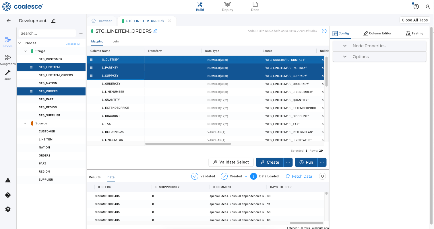
-
Let’s rename some of the columns in our node for readability. Click Column Name to sort. Press and hold the Shift key to multi-select all columns that begin with the L_ prefix. Then right click and select Bulk Edit from the drop down menu.
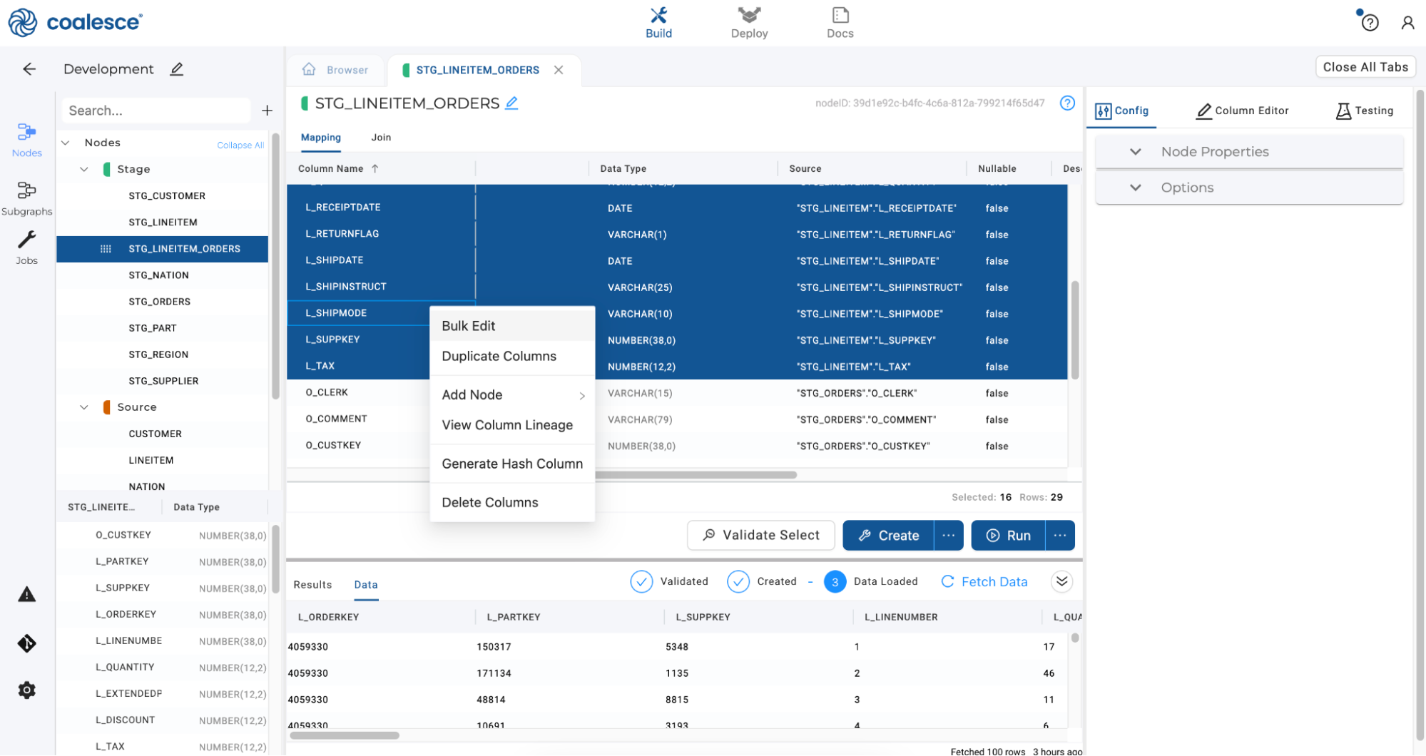
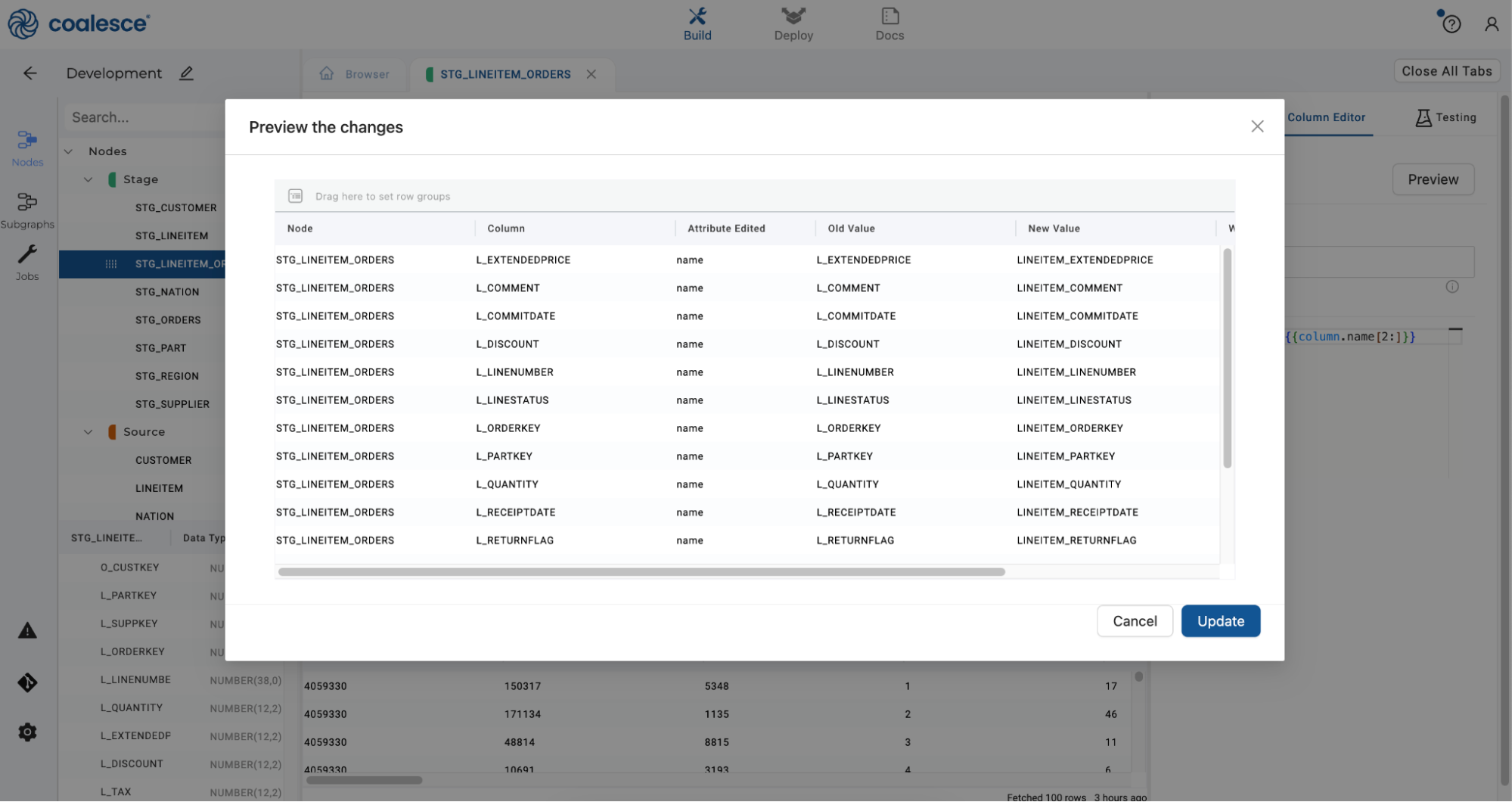
-
Select Column Name as your attribute and enter the code
LINEITEM_{{column.name[2:]}}to rename the columns. This particular Jinja code snippet will concatenate the prefix and remove the first 2 characters from the original column name.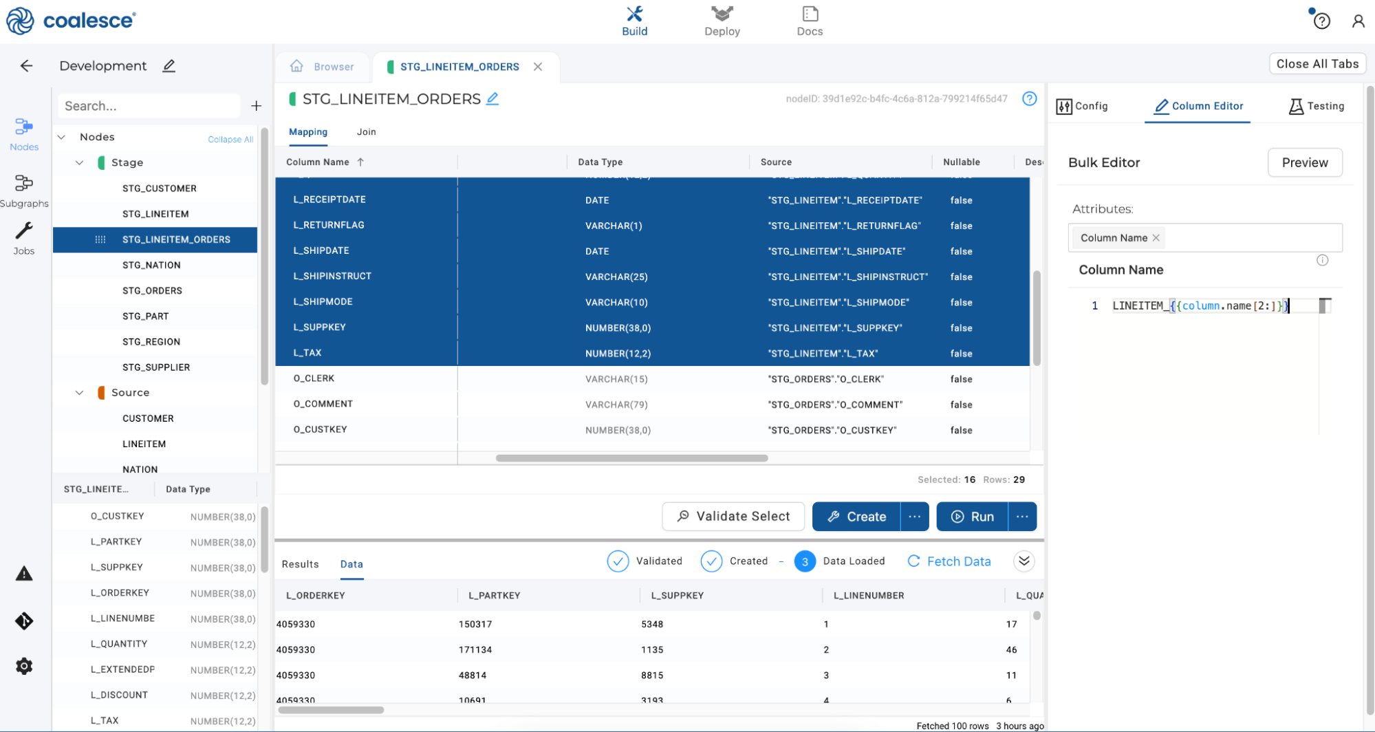
-
Repeat this process by bulk renaming all columns with an O_ prefix using the code
ORDER_{{column.name[2:]}}.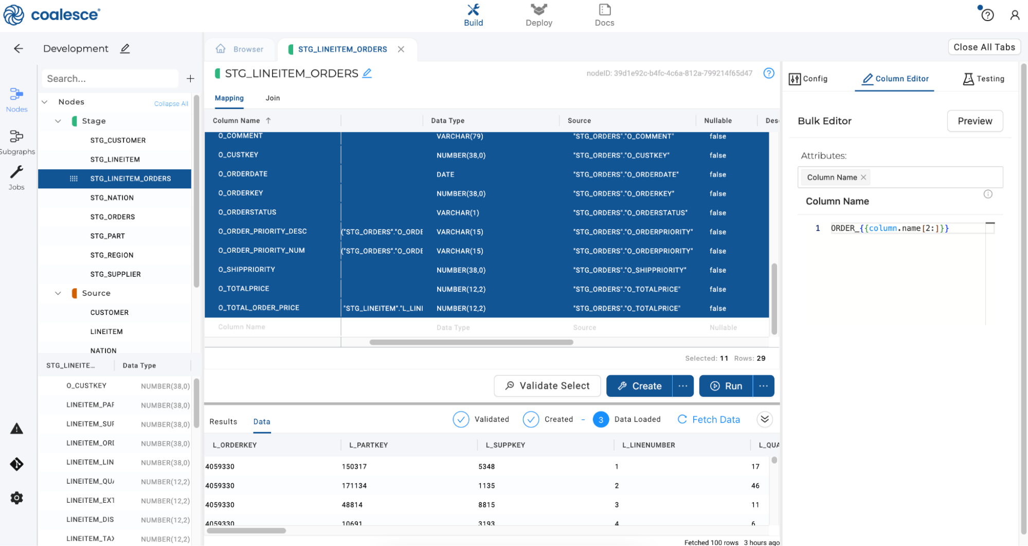
-
Click Preview to check your renaming rule, and then press Update to apply it to your selected columns.
-
Click Create and Run to update your
STG_LINEITEM_ORDERSnode.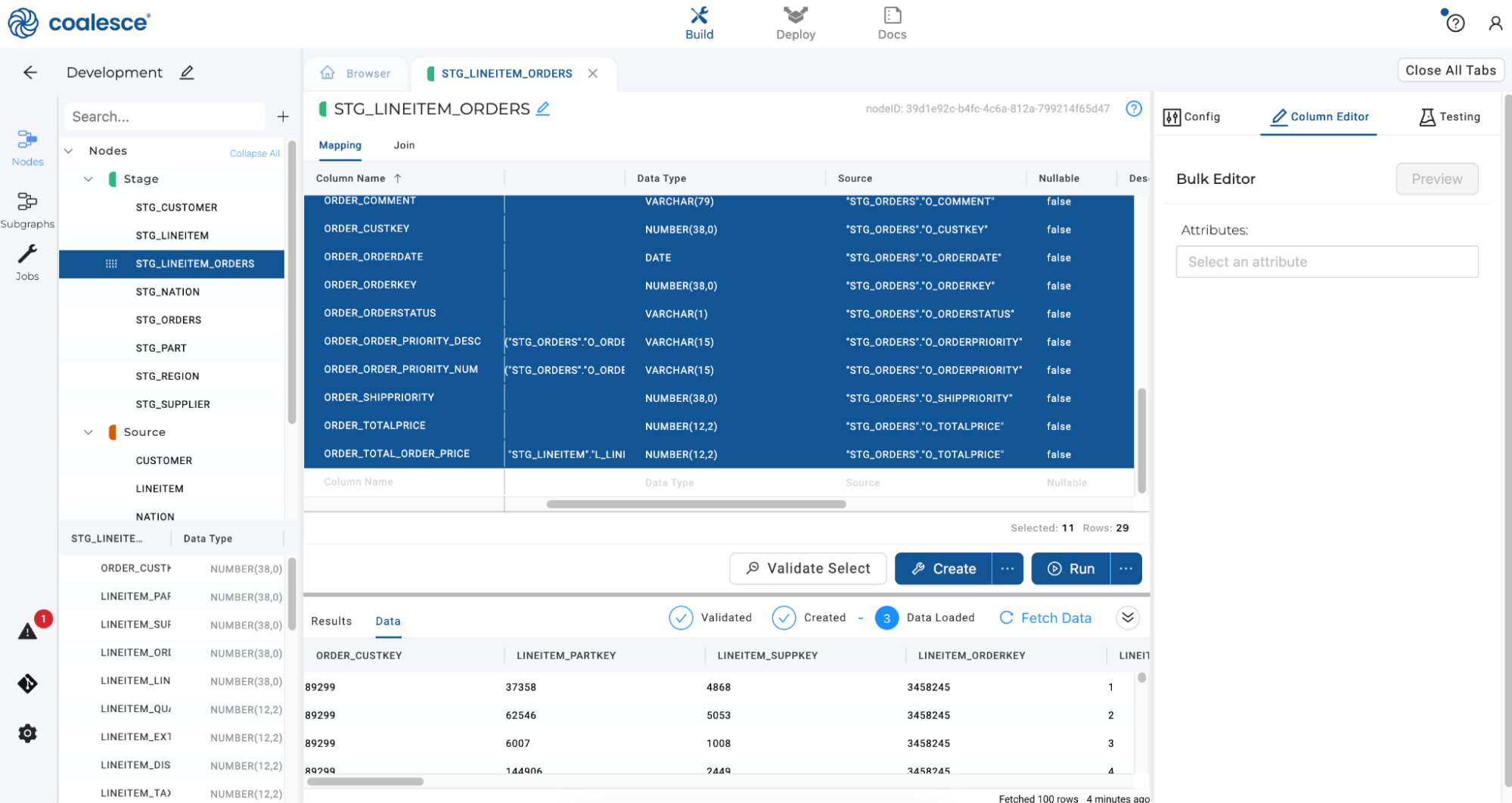
-
Now let’s create a Dimension node for each of these foreign key columns by navigating back to the Browser tab. Press the Shift key and select
STG_CUSTOMER,STG_SUPPLIERandSTG_PARTsource nodes on the graph. Then right click and select Add Node > Dimension.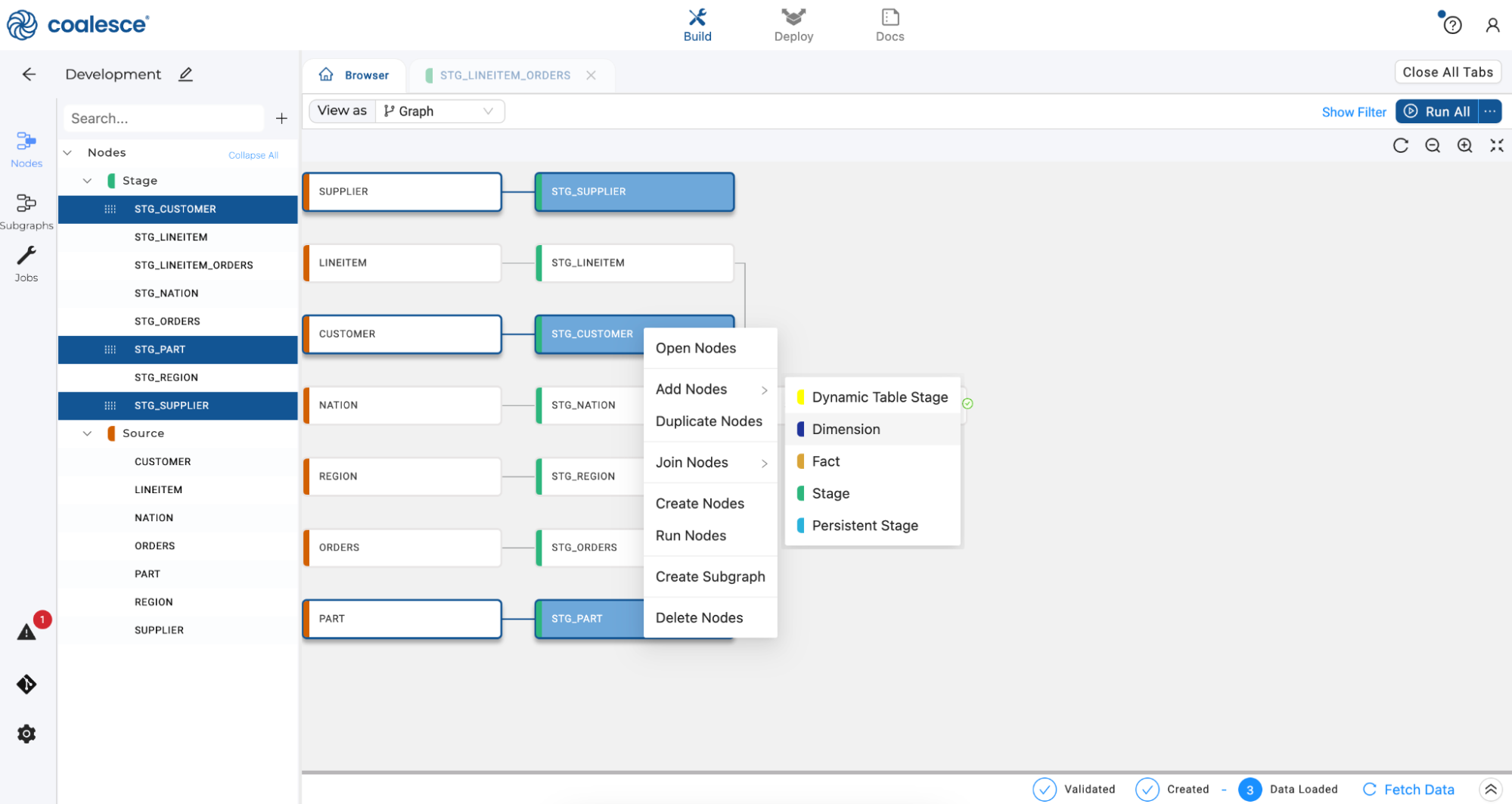
-
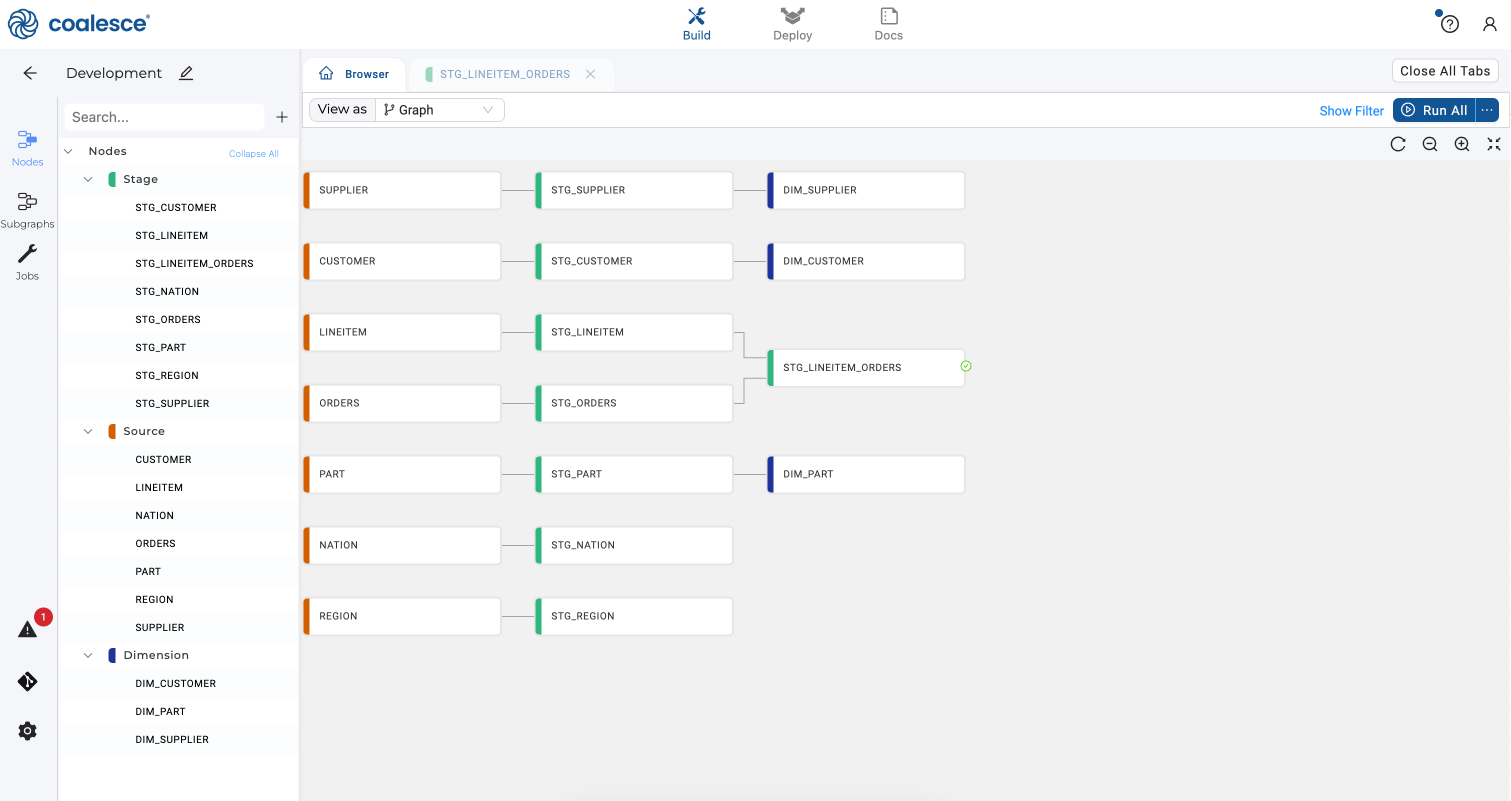
A Dimension node will appear for each of your selected Stage nodes. Under the Run All button, click the first icon to optimize the layout of your graph.
-
Double click on your new DIM_PART node to open up the Node Editor. In the Config section on the right hand side of the screen, click to expand Options. Under Business Key, check the box next to
P_PARTKEYand press the > button to select it as your business key. This will remain a Type 1 dimension, so we will not select columns for change tracking over time.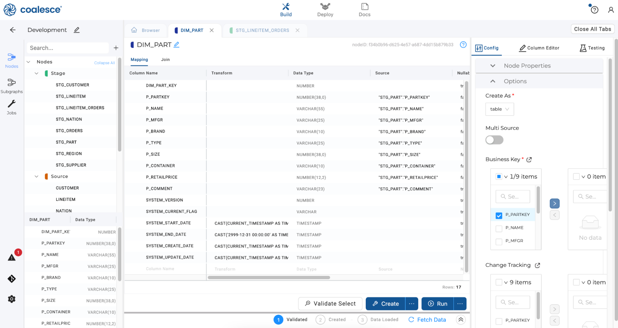
-
Return to the Browser tab and double click on the
DIM_CUSTOMERnode. In the Config section of your editor, expand Options and selectC_CUSTKEYas your business key.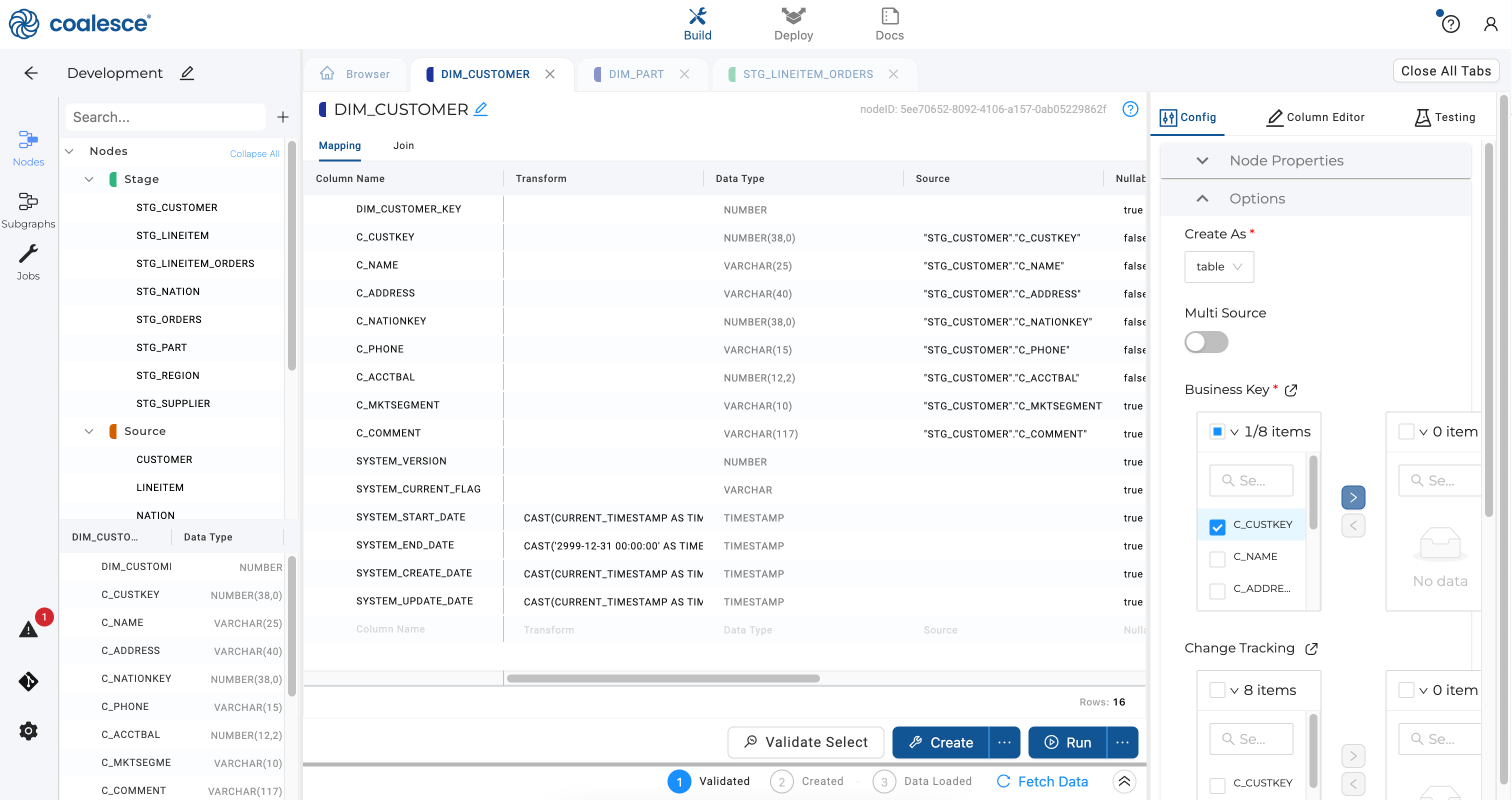
To create a Type 2 dimension, select the
C_NAMEandC_ADDRESScolumns under Change Tracking to track changes to these columns over time.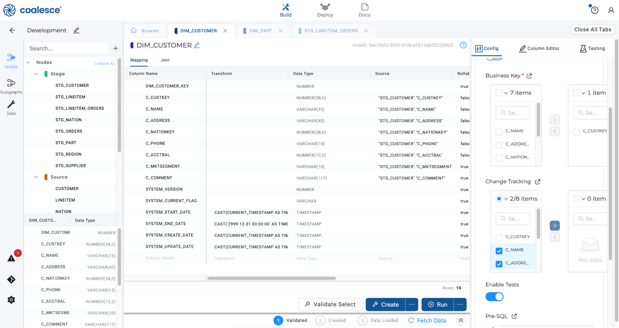
-
Return to the Browser tab once more and double click to open up the
DIM_SUPPLIERnode. SelectS_SUPPKEYas your business key to create a Type 1 dimension.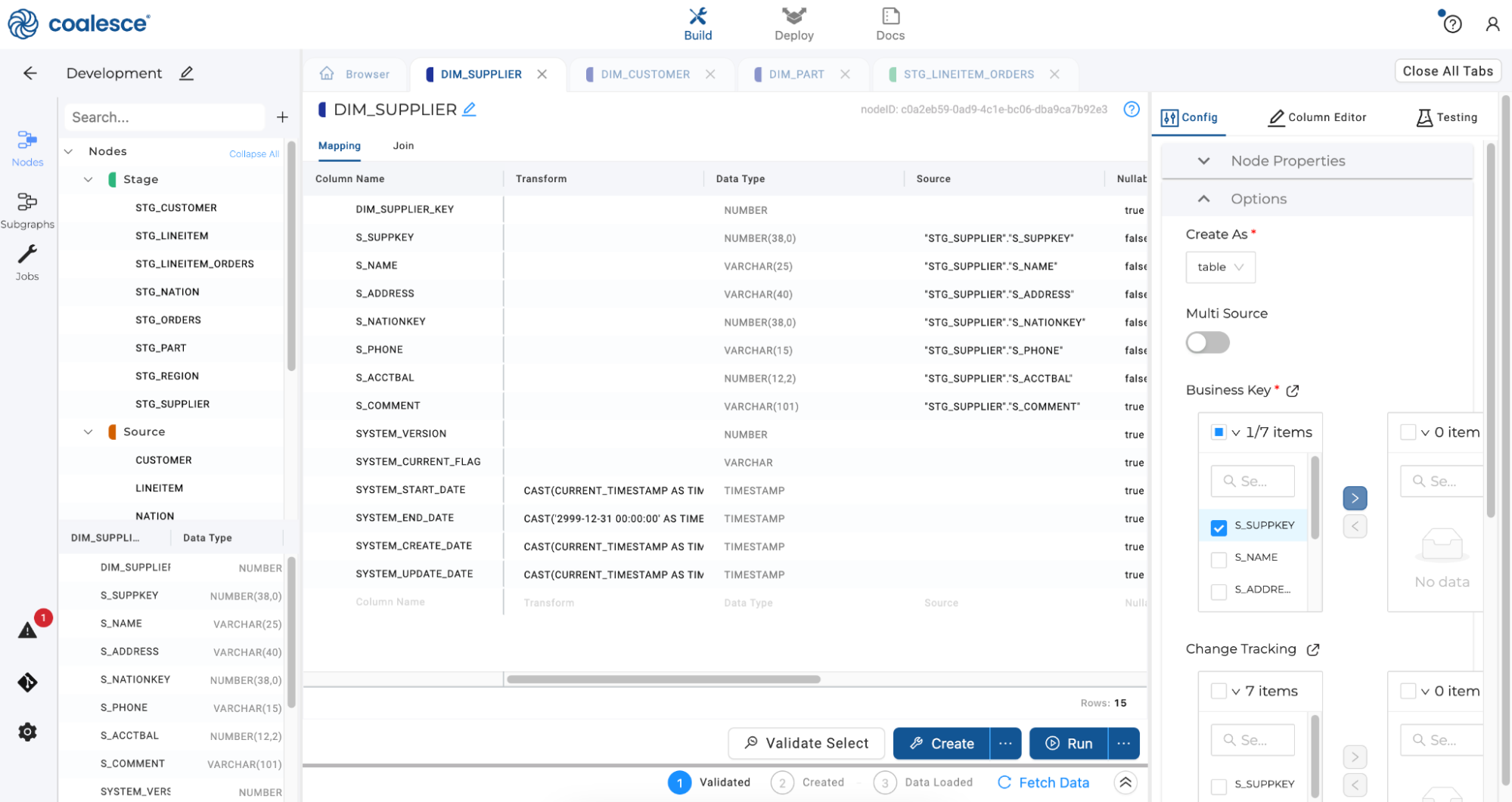
-
Return to your graph and click Create All and Run All in the upper right hand corner.
Bulk Editing Columns
Now let’s apply a bulk transformation to some of the columns in your DIM_CUSTOMER node. Double click on DIM_CUSTOMER in your graph to open up your Node Editor.
-
In the Mapping grid, click twice on Data Type to bring all VARCHAR columns to the top of the grid. Press and hold the Shift key to multi-select all the VARCHAR columns beginning with the
C_prefix. Right click on your selections and click on Bulk Edit in the dropdown menu.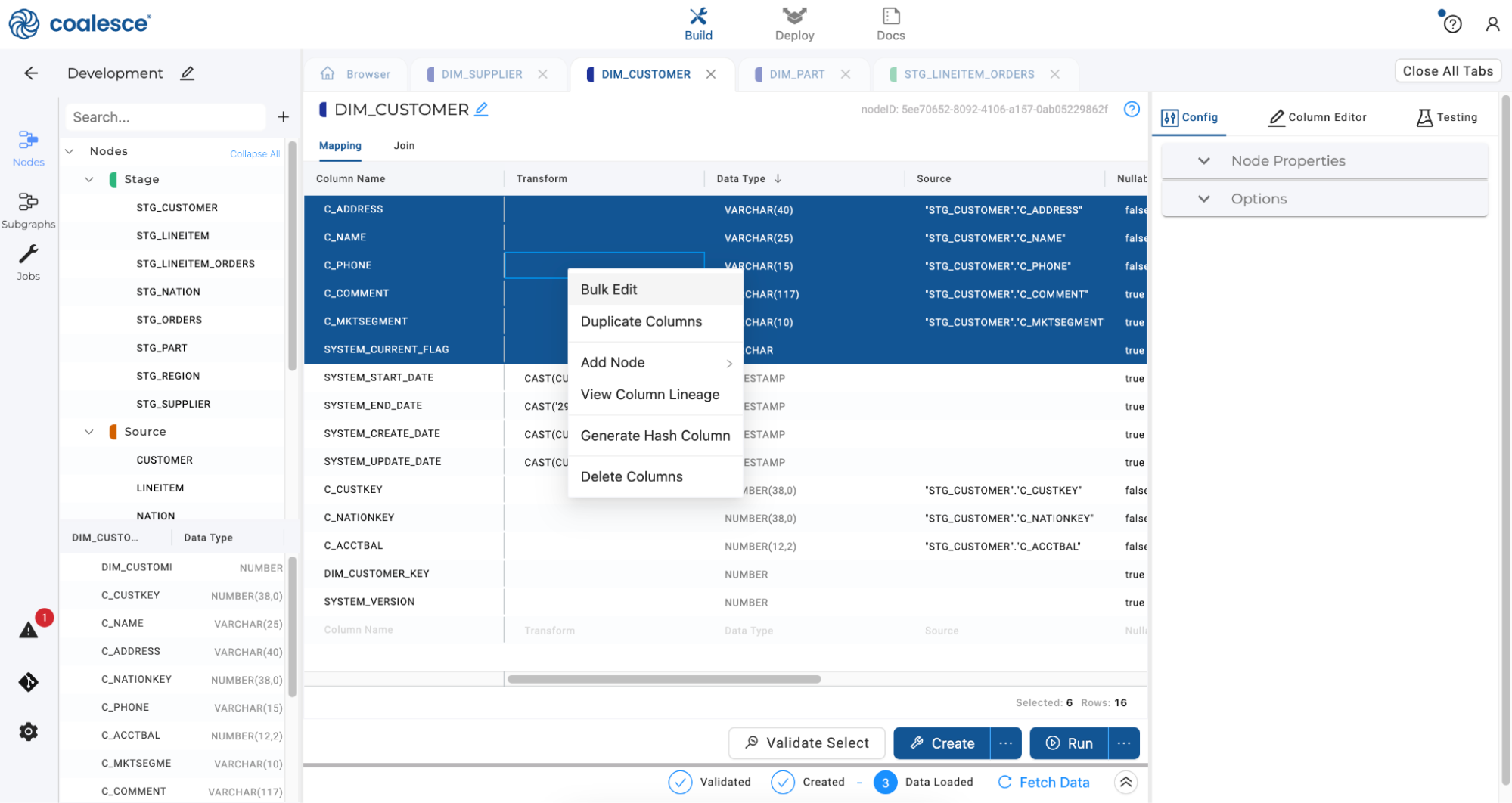
-
Click on the Column Editor on the right hand side of the screen. Select Data Type and Transform under Attributes. Clarify the Data Type as STRING and enter the transformation
UPPER({{SRC}})in the Transform field.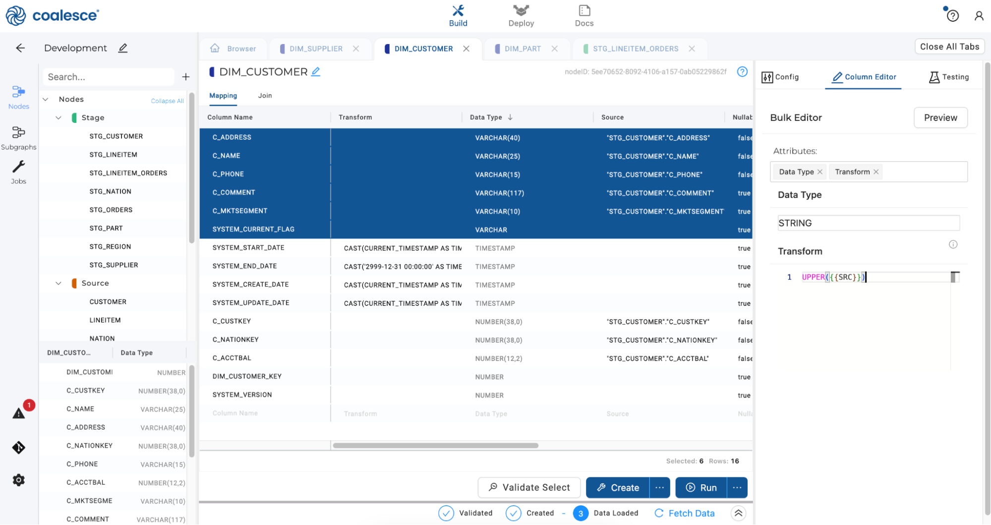
-
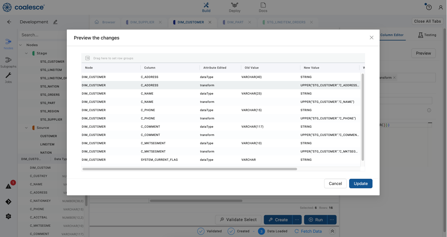
Click the Preview button and then press Update to apply the bulk transformation.
-
Return to the Browser tab and right click the
STG_LINEITEM_ORDERSnode to create a new Stage node, which will be a lookup table for our Dimension nodes.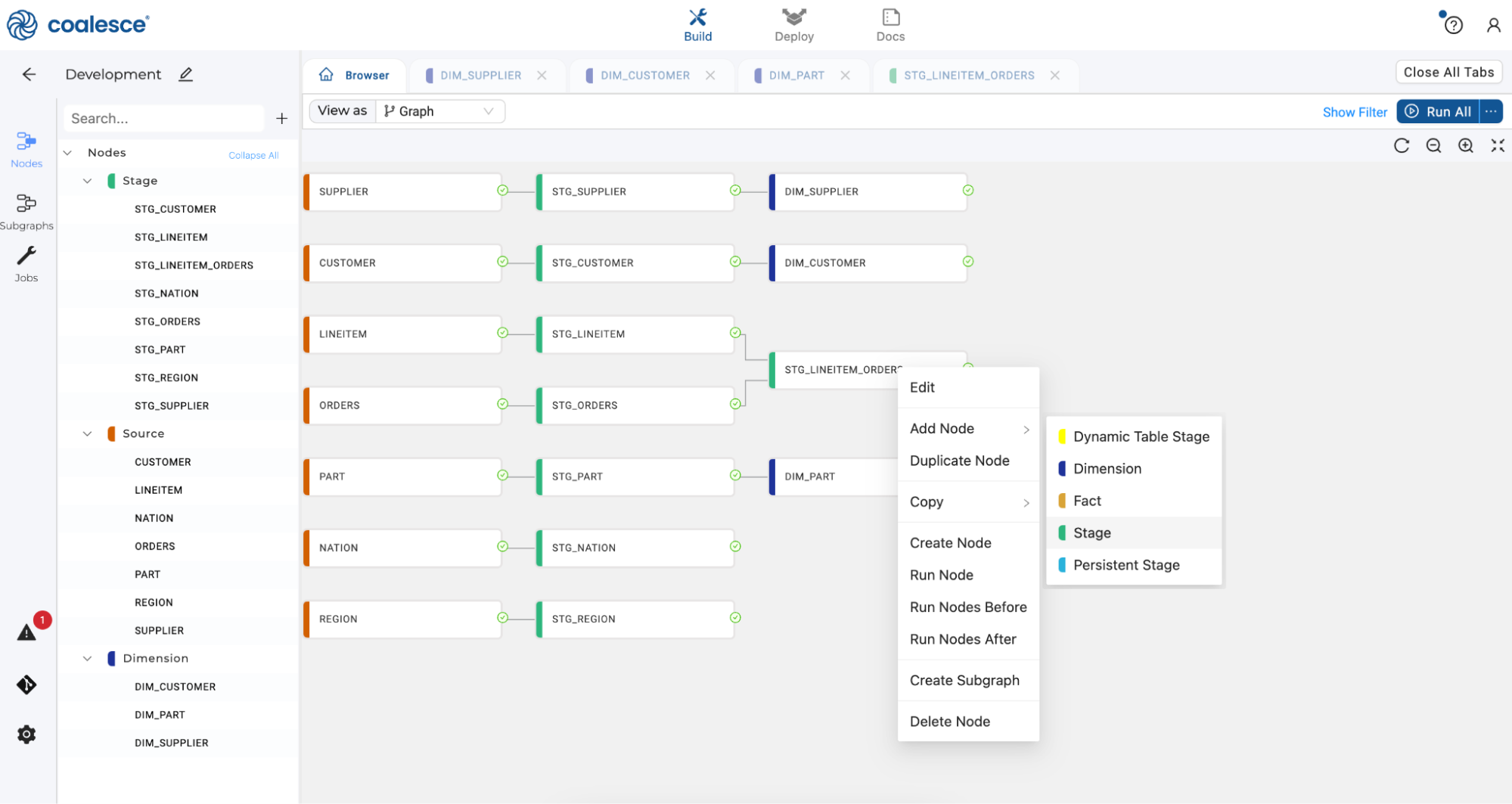
-
Open the new Stage node and rename it
STG_LINEITEM_ORDERS_DIM_LOOKUPin the Node Editor. On the left hand side of the screen in the Node and Column selector, select theDIM_CUSTOMERnode. Drag theDIM_CUSTOMER_KEYcolumn from the column selector over to the bottom of your Mapping grid.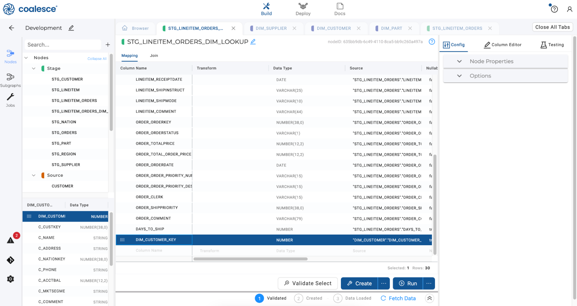
-
Repeat this action by selecting the
DIM_PARTnode and dragging theDIM_PART_KEYcolumn into the Mapping grid.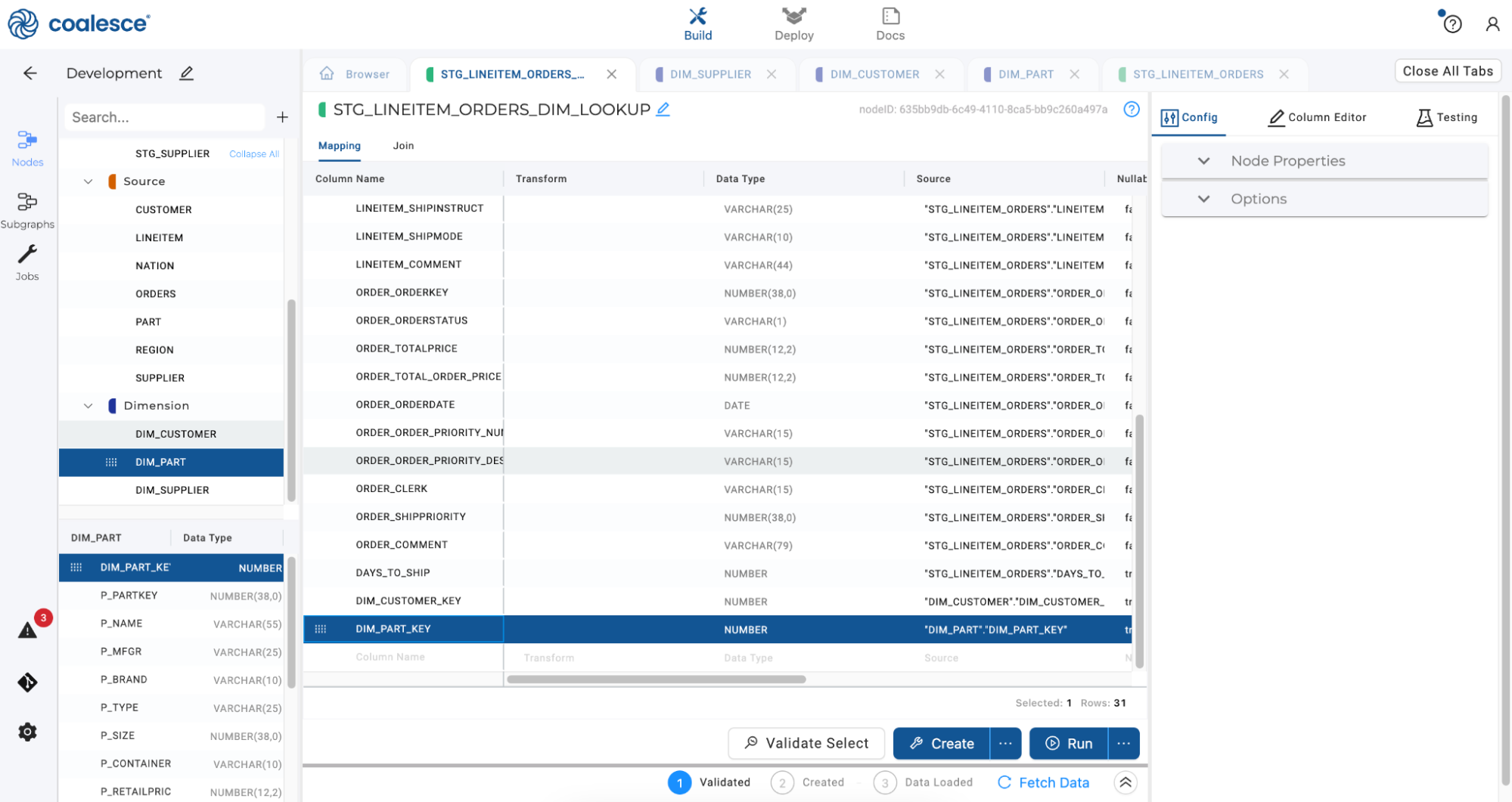
-
Repeat this action once more by selecting the
DIM_SUPPLIERnode and dragging theDIM_SUPPLIER_KEYcolumn into the Mapping grid.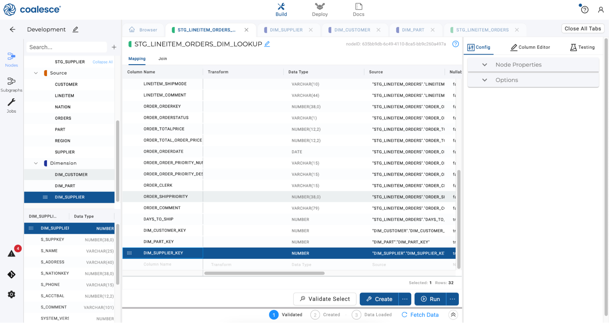
-
Select the Join tab and delete the existing code shown.
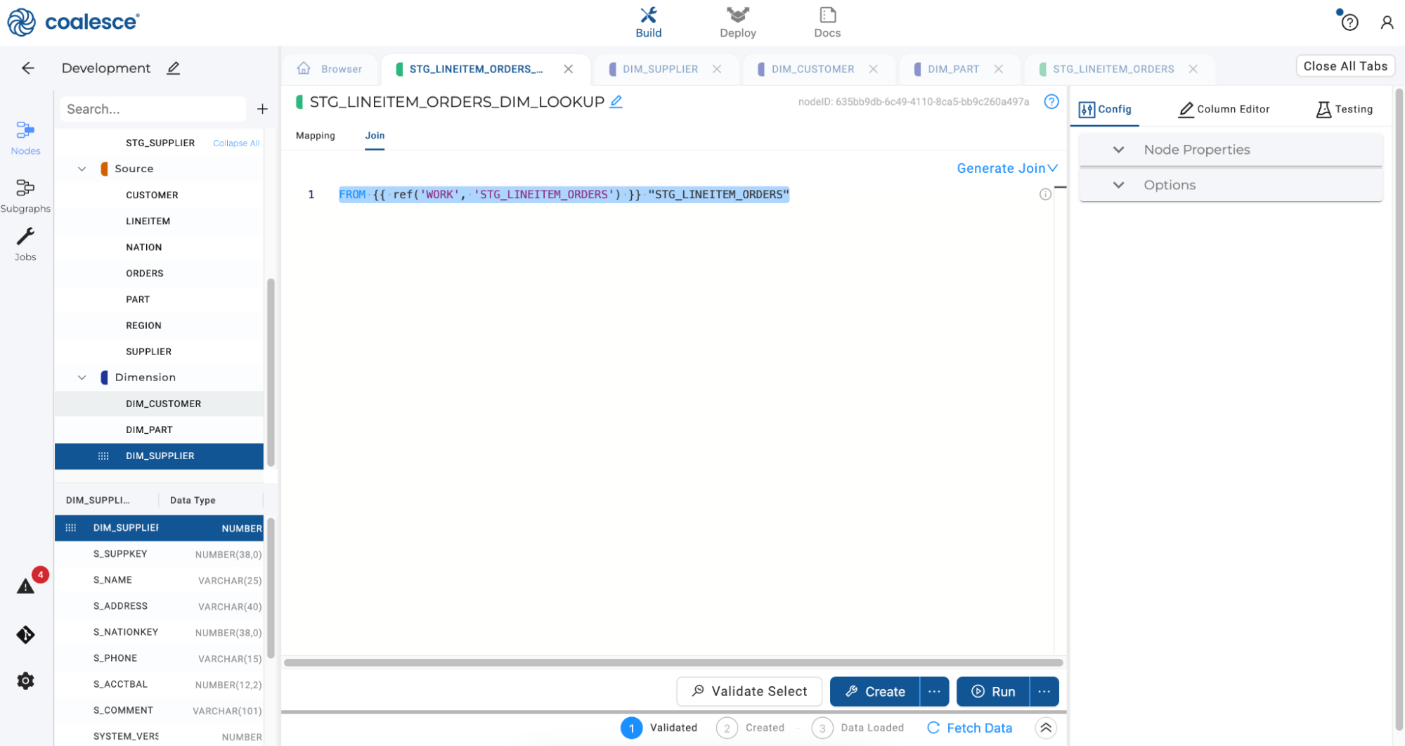
-
Click Generate Join and then Copy to Editor to automatically import your join statement.
Copy to editorFROM {{ ref('WORK', 'STG_LINEITEM_ORDERS') }}"STG_LINEITEM_ORDERS"LEFT JOIN {{ ref('WORK', 'DIM_CUSTOMER') }}"DIM_CUSTOMER"ON "STG_LINEITEM_ORDERS"./*COLUMN*/ = "DIM_CUSTOMER"."C_CUSTKEY"LEFT JOIN {{ ref('WORK', 'DIM_PART') }} "DIM_PART"ON "STG_LINEITEM_ORDERS"./*COLUMN*/ = "DIM_PART"."P_PARTKEY"LEFT JOIN {{ ref('WORK', 'DIM_SUPPLIER') }}"DIM_SUPPLIER"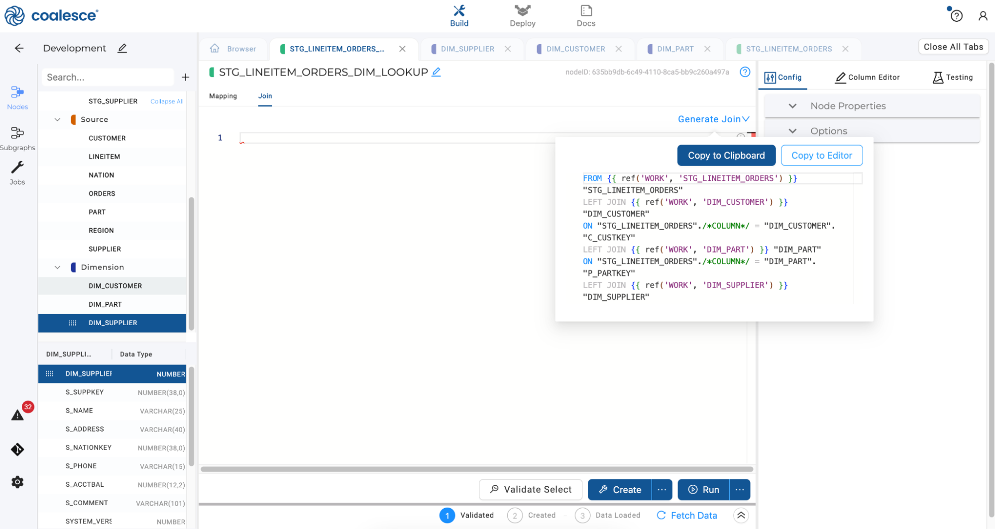
-
Manually resolve the join by adding
ORDER_CUSTKEY,LINEITEM_PARTKEYandLINEITEM_SUPPKEYinto the empty column names. Then click the Create and Run buttons to create and populate yourSTG_LINEITEM_ORDERS_DIM_LOOKUPnode.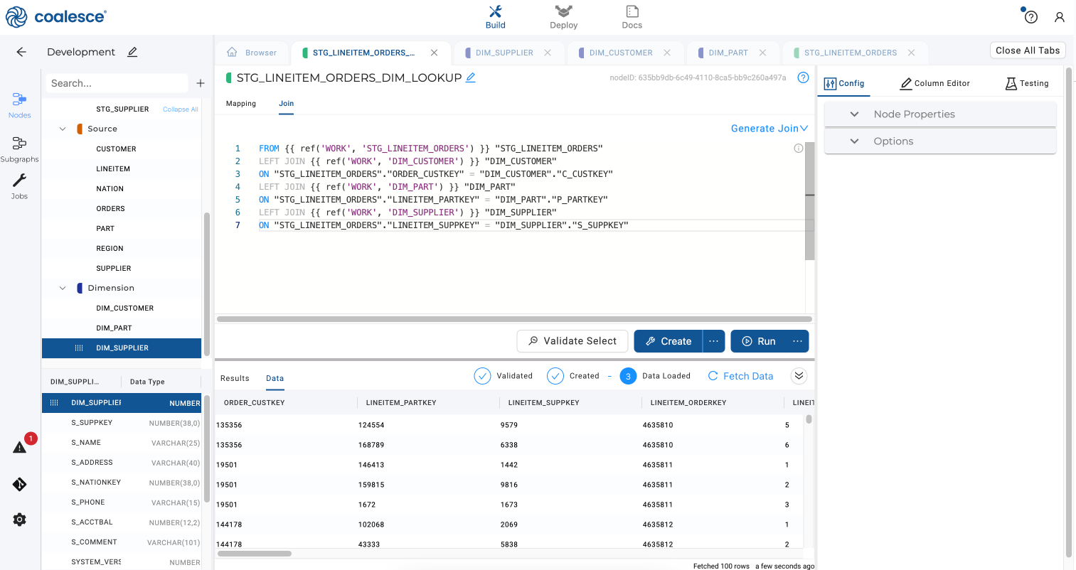
Note that If this source data had changed for customer, we would just need an additional line of code in the join.
Creating and Updating Fact Nodes
Now let’s create a Fact node. Fact nodes represent Coalesce's implementation of a Kimball Fact Table, which consists of the measurements, metrics, or facts of a business process and is typically located at the center of a star or Snowflake schema surrounded by dimension tables.
-
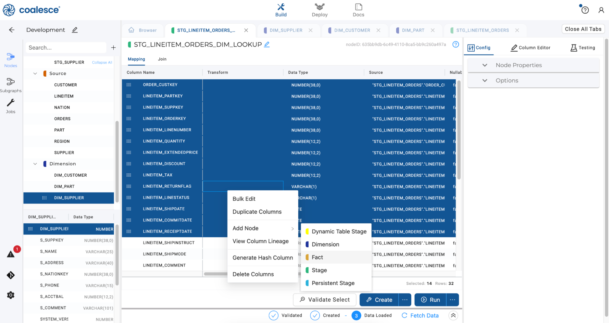
Click on Mapping and then click on Data Type. Hold the Shift key and select the NUMBER and DATE columns only. Then right click to create a Fact node from just these columns, as Fact tables typically only contain measurements (as opposed to text, which would potentially be in a Dimension node).
-
Once your new Fact node has opened, rename it to
FCT_ORDER_DETAILS. Return to your Browser tab and click Create and then Run to populate it with data.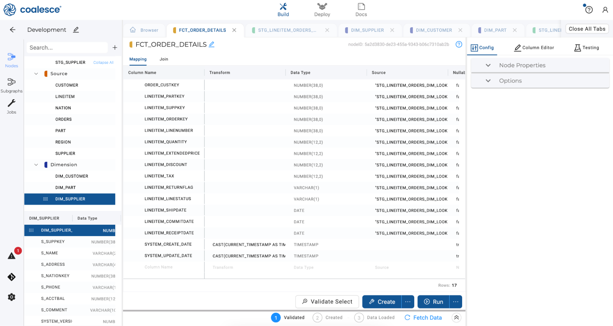
Congratulations. You have now built out a small data mart.
Propagating Changes Across Pipelines
Of course, business requirements are always changing and the business has now decided that they want to include supply costs as part of their analysis. Let’s explore how you can manage your pipeline under these evolving circumstances.
-
Click the + button next to the Search bar on the left side of the Browser tab and select Add Sources.

-
Expand the sample dataset and select the PARTSUPP source. Then click the Add 1 source button.

-
Double click on the new PARTSUPP source node to open it. You’ll see two columns,
PS_AVAILQTYandPS_SUPPLYCOST, that need to appear in theFCT_ORDER_DETAILStable.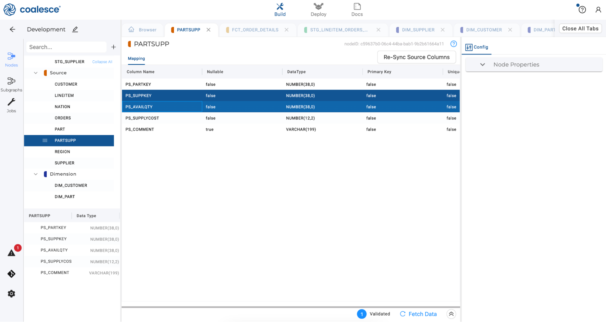
-
Return to the Browser and double click on your
STG_LINEITEMnode to open it. In the left hand portion of the Mapping grid, select the PARTSUPP node. Select thePS_AVAILQTYandPS_SUPPLYCOSTcolumns and drag them into the bottom of the Mapping grid, effectively moving these columns into yourSTG_LINEITEMnode.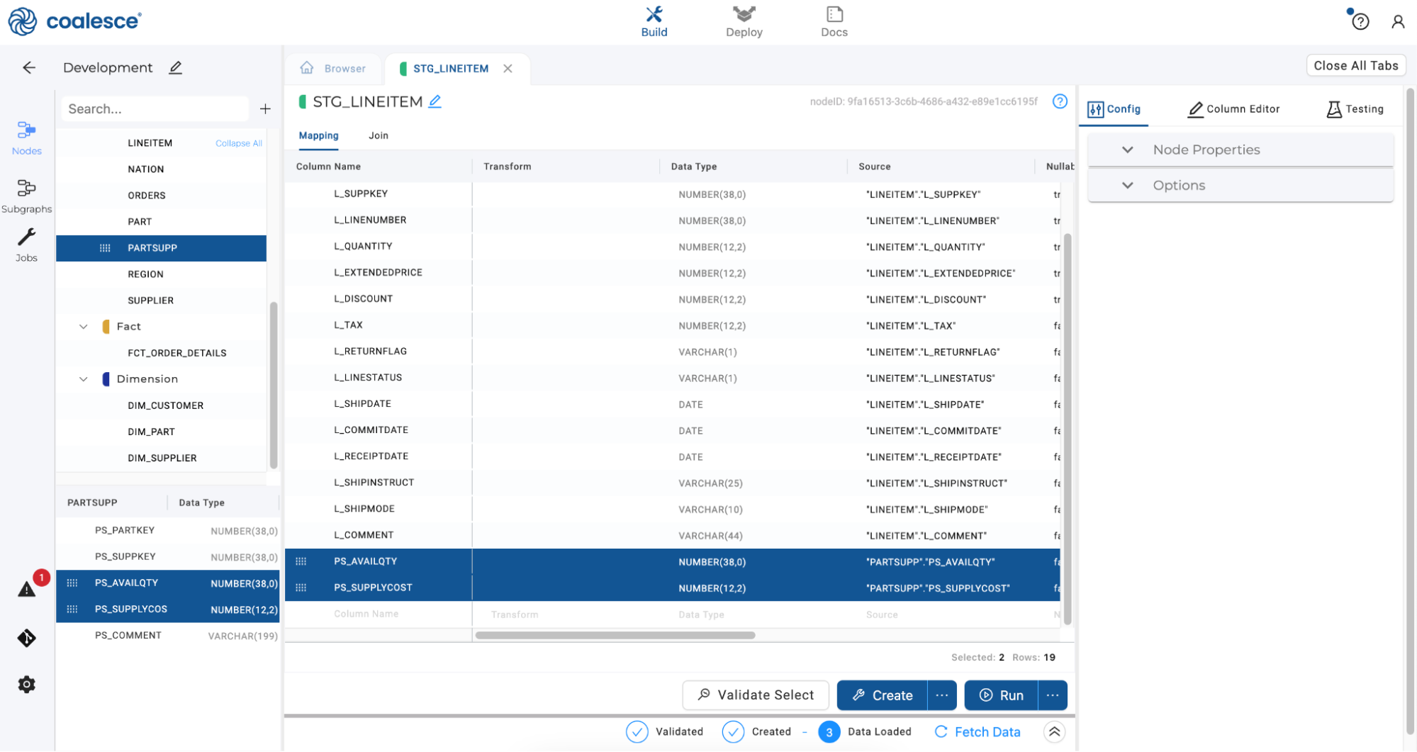
-
Click on the Join tab and then click on Generate Join. Copy the last line to the Join tab and complete the statement with the
L_PARTKYandPS_PARTKEYcolumns to joinPARTSUPPwithSTG_LINEITEM.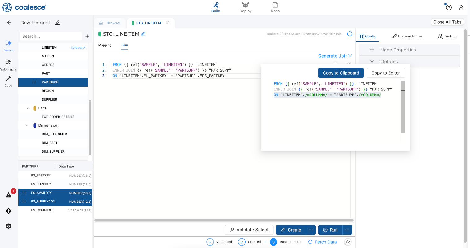
-
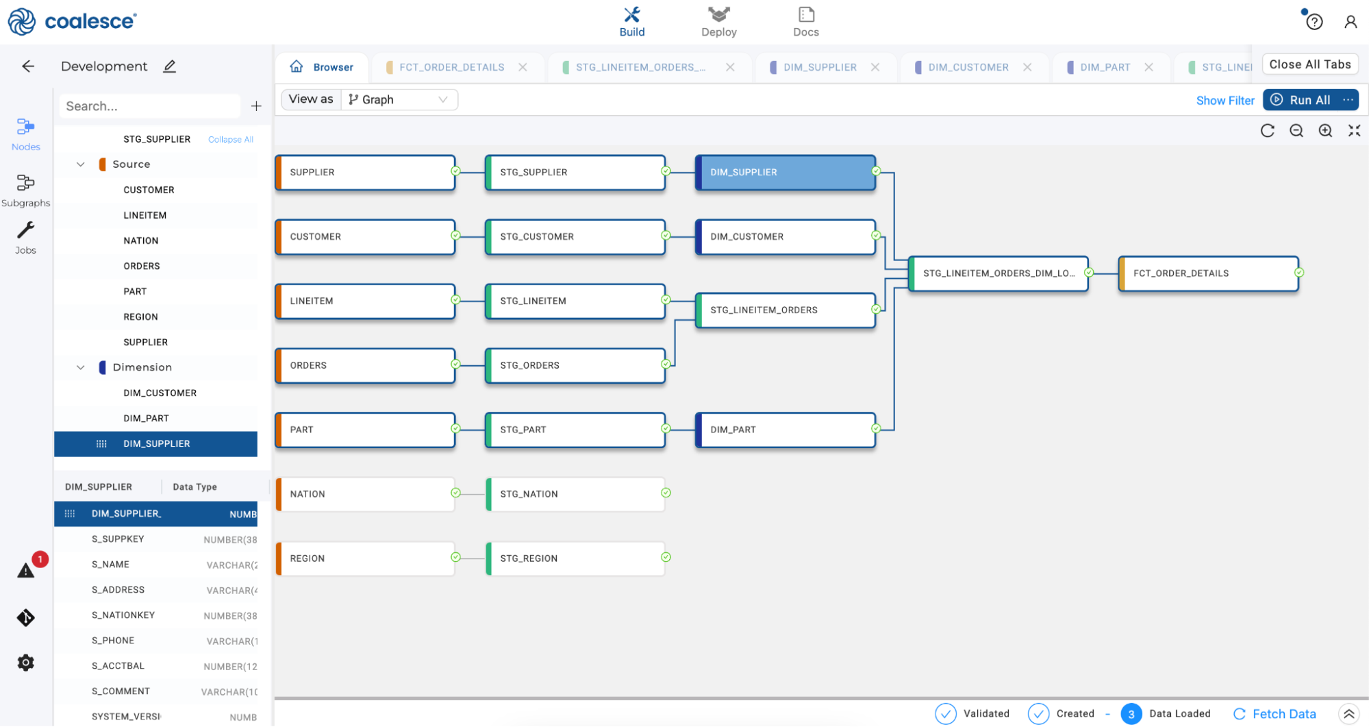
Return to the Browser tab and click the Create and Run buttons, and then click the spiral icon to optimize your Graph.
-
Now let’s take a look at our column lineage and ensure that all of our columns are carried through our pipeline. Switch back to your
STG_LINEITEMnode and select thePS_AVAILQTYandPS_SUPPLYCOSTcolumns. Then right click and select View Column Lineage from the dropdown menu.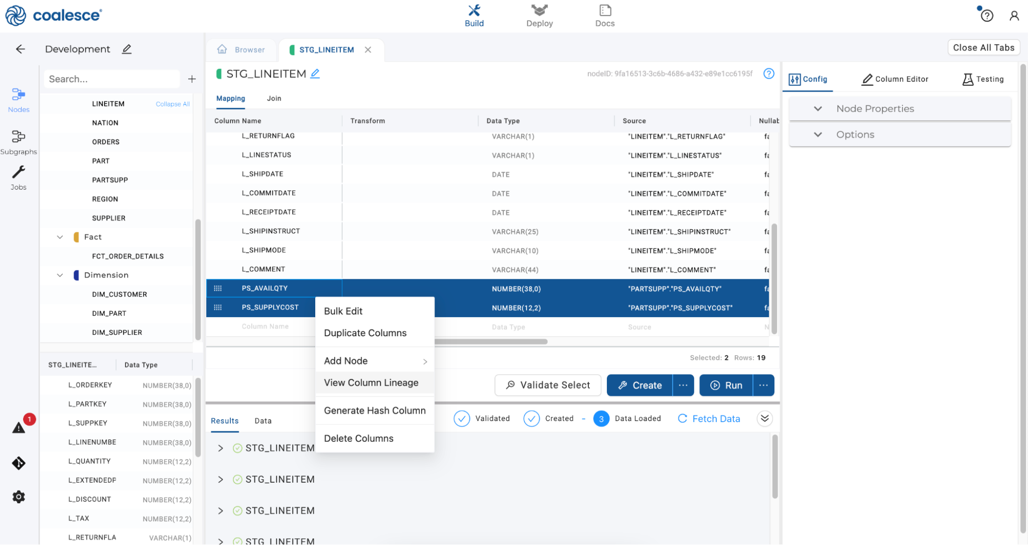
-
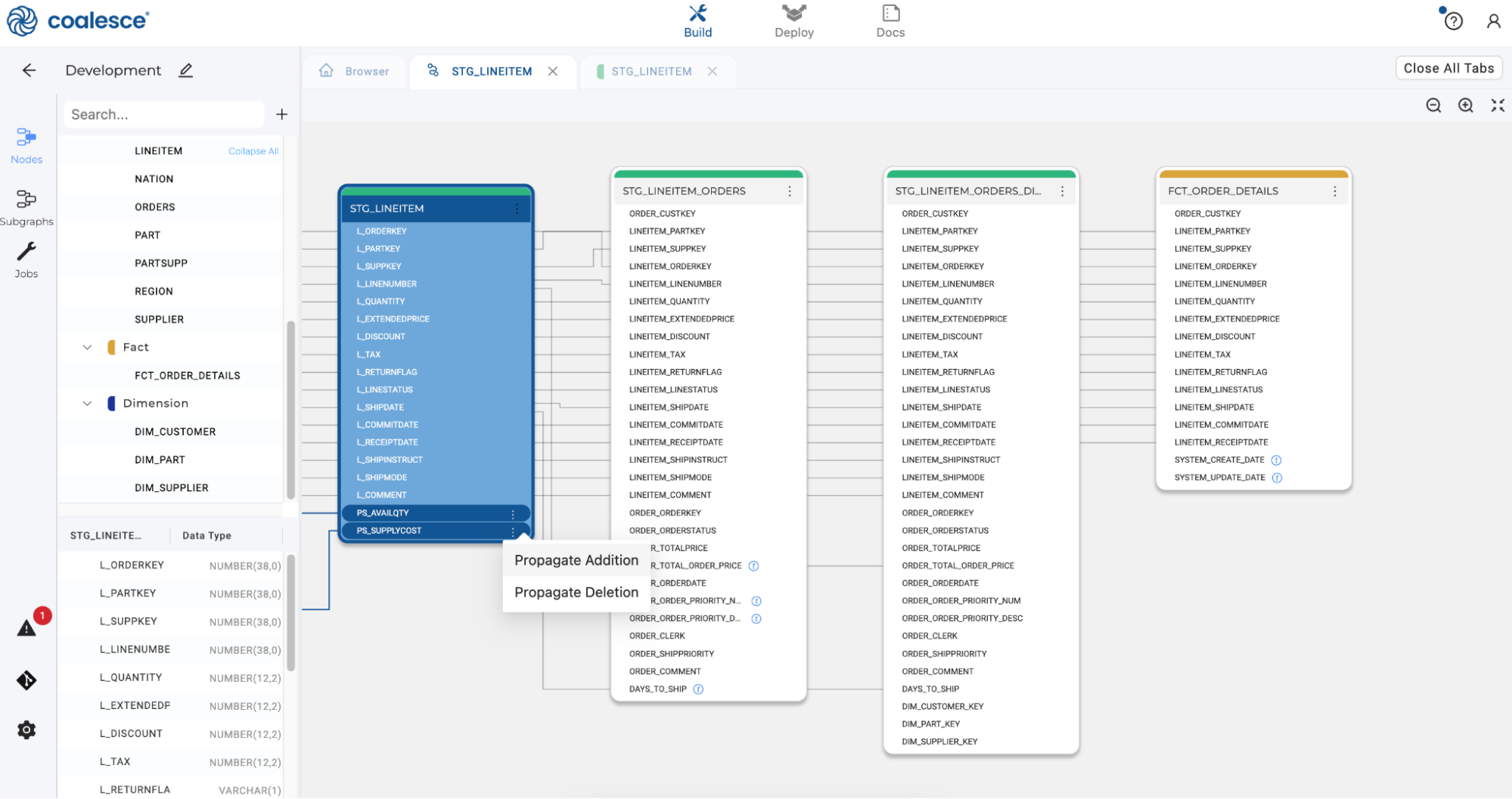
Once in the Column Lineage view, select both columns and click the ellipses to select Propagate Addition. This will allow you to propagate these columns to the downstream nodes in your pipeline.
-
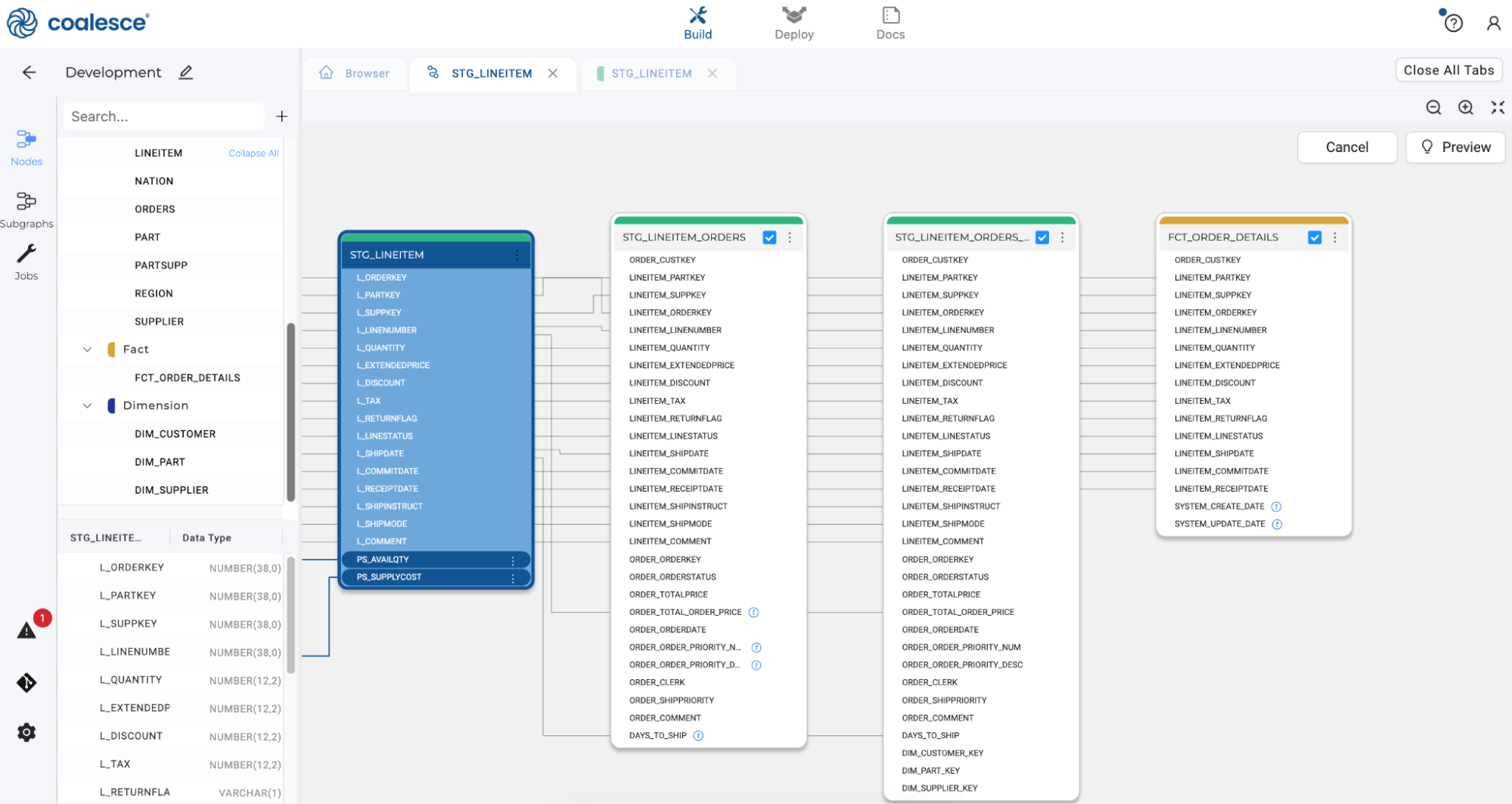
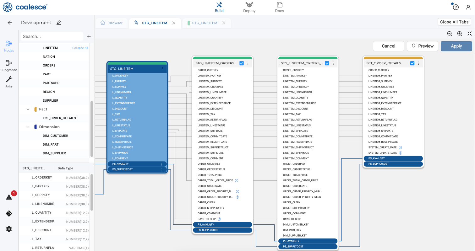
Check the boxes to add these columns to the last two successor nodes in your pipeline.
-
Click the Preview button to confirm that your two columns have been added to the bottom of each successor node. Then Click Apply and Confirm to propagate your additions.
-
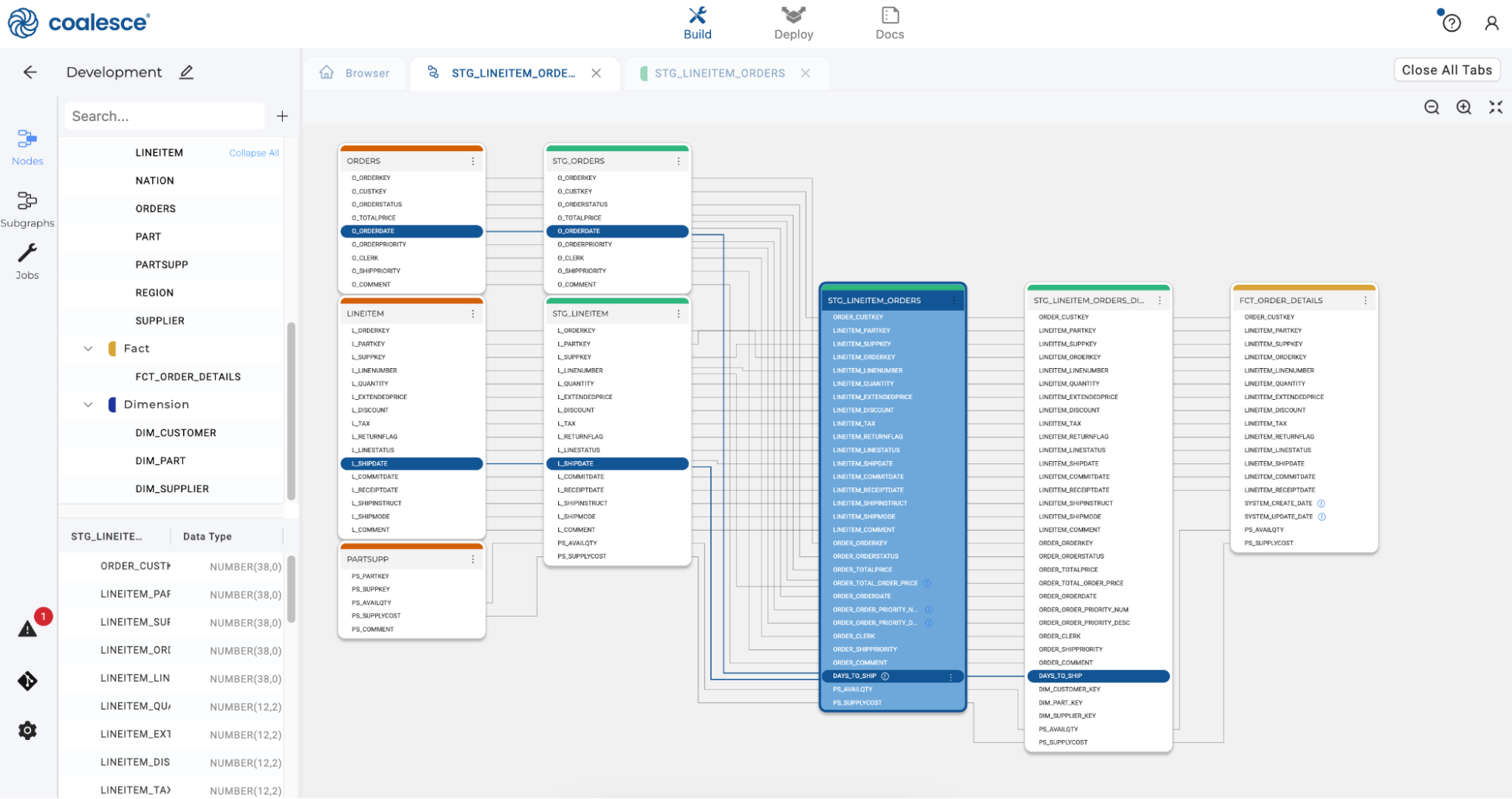
By clicking on the DAYS_TO_SHIP column, you can view the concatenation and split lineage of this column. Then return to the Browser tab and click the Run All button to refresh your pipeline.
Optimizing, Running and Validating Your DAG
-
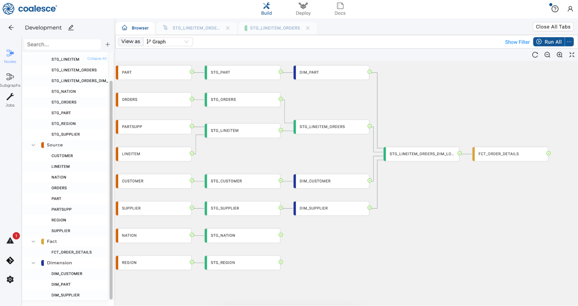
Return to the Browser tab of the Build Interface. Click the
 icon under Run All to visually optimize the organization of your nodes.
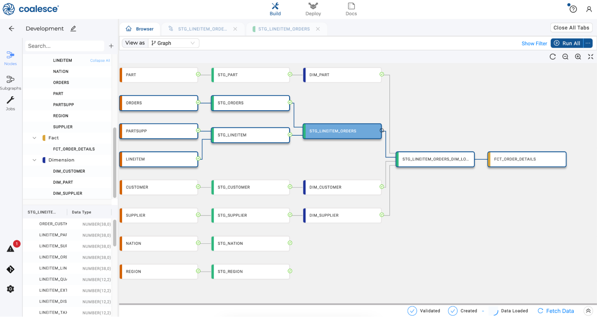
-
From the Run All dropdown, select Validate Create All and confirm there are no errors with the create statements in your pipeline. Upon confirmation, execute a Create All. Repeat these validation and execution steps with Run All.
-
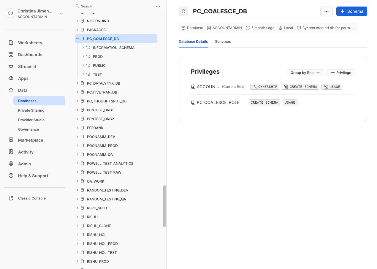
Switch to your Snowflake account and view the tables and data within the Snowflake platform to ensure everything is as intended. You will find your build in PC_COALESCE_DB.PUBLIC (database.schema) as shown in the screenshot below.
Conclusion and Next Steps
Congratulations on completing this entry-level lab exercise. You've mastered the basics of Coalesce and are now equipped to venture into our more advanced features. Be sure to reference this exercise if you ever need a refresher.
We encourage you to continue working with Coalesce by using it with your own data and use cases and by using some of the more advanced capabilities not covered in this lab.
What We’ve Covered
- How to navigate the Coalesce interface
- How to add data sources to your graph
- How to prepare your data for transformations with Stage nodes
- How to join tables
- How to apply transformations to individual and multiple columns at once
- How to build out Dimension and Fact nodes
- How make and propagate changes to your data across pipelines
Continue with your free trial by loading your own sample or production data and exploring more of Coalesce’s capabilities with our documentation and resources.
Additional Resources
Reach out to our sales team at coalesce.io or by emailing sales@coalesce.io to learn more.