Getting Started Building Pipeline on Databricks with Coalesce

Overview

1. This entry-level Hands-On Lab exercise is designed to help you master the basics of Coalesce. In this lab, you’ll explore the Coalesce interface, learn how to easily transform and model your data with our core capabilities, and understand how to deploy and refresh version-controlled data pipelines.

What You’ll Need

• A Databricks trial account
• A Coalesce trial account
• Basic knowledge of SQL, database concepts, and objects
• The Google Chrome Browser

What You’ll Build

A Directed Acyclic Graph (DAG) representing a basic star schema in Databricks

What You’ll Learn

• How to navigate the Coalesce interface
• How to add data sources to your graph
• How to prepare your data for transformations with Stage nodes
• How to join tables
• How to apply transformations to individual and multiple columns at once
• How to build out Dimension and Fact nodes
• How to make changes to your data and propagate changes across pipelines
• By completing the steps we’ve outlined in this guide, you’ll have mastered the basics of Coalesce and can venture into our more advanced features.

About Coalesce

Coalesce enables data teams to develop and manage data pipelines in a sustainable way at enterprise scale and collaboratively transform data without the traditional headaches of manual, code-only approaches.

What Can You Do With Coalesce?

• With Coalesce, you can:
• Develop data pipelines and transform data as efficiently as possible by coding as you like and automating the rest, with the help of an easy-to-learn visual interface
• Work more productively with customizable templates for frequently used transformations, auto-generated and standardized SQL, and full support for Databricks functionality
• Analyze the impact of changes to pipelines with built-in data lineage down to the column level
• Build the foundation for predictable DataOps through automated CI/CD workflows and full Git integration
• Ensure consistent data standards and governance across pipelines, with data never leaving your Databricks instance

How Is Coalesce Different?

Coalesce’s unique architecture is built on the concept of column-aware metadata, meaning that the platform collects, manages, and uses column- and table-level information to help users design and deploy data warehouses more effectively. This architectural difference gives data teams the best that legacy ETL and code-first solutions have to offer in terms of flexibility, scalability, and efficiency.

Data teams can define data warehouses with column-level understanding, standardize transformations with data patterns (templates) and model data at the column level.

Coalesce also uses column metadata to track past, current, and desired deployment states of data warehouses over time. This provides unparalleled visibility and control of change management workflows, allowing data teams to build and review plans before deploying changes to data warehouses.

Core Concepts in Coalesce

Multi-Platform

Coalesce supports multiple data platforms as the target of your work. As you will be using a trial Coalesce account, your basic database settings will be configured in the first few sections of the lab guide.

Organization

A Coalesce organization is a single instance of the UI, set up specifically for a single prospect or customer. It is set up by a Coalesce administrator and is accessed via a username and password. By default, an organization will contain a single Project and a single user with administrative rights to create further users.

Projects

Projects provide a way of completely segregating elements of a build, including the source and target locations of data, the individual pipelines and ultimately the Git repository where the code is committed. Therefore teams of users can work completely independently from other teams who are working in a different Coalesce Project.

Each Project requires access to a Git repository and Databricks account to be fully functional. A Project will default to containing a single Workspace, but will ultimately contain several when code is branched.

Workspaces VS Environments

A Coalesce Workspace is an area where data pipelines are developed that point to a single Git branch and a development set of Databricks schemas. One or more users can access a single Workspace. Typically there are several Workspaces within a Project, each with a specific purpose (such as building different features). Workspaces can be duplicated (branched) or merged together.

A Coalesce Environment is a target area where code and job definitions are deployed to. Examples of an environment would include QA, UAT, and Production.

It isn’t possible to directly develop code in an Environment, only deploy to there from a particular Workspace (branch). Job definitions in environments can only be run via the CLI or API (not the UI). Environments are shared across an entire project, therefore the definitions are accessible from all workspaces. Environments should always point to different target schemas (and ideally different databases), than any Workspaces.

About This Guide

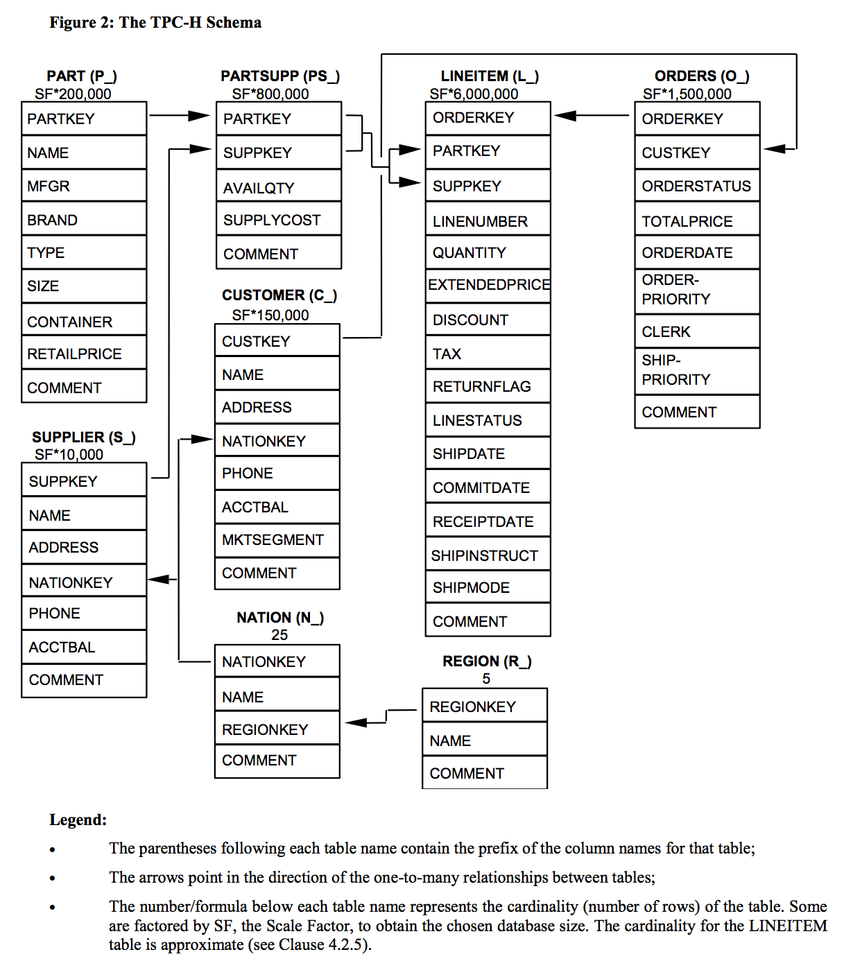
The exercises in this guide use the sample data provided with Databricks trial accounts. This data is focused on fictitious commercial business data including supplier, customer, and orders information.

Before You Start

1. To complete this lab, please create free trial accounts with Databricks and Coalesce by following the steps below. You have the option of setting up Git-based version control for your lab, but this is not required to perform the following exercises. Please note that none of your work will be committed to a repository unless you set Git up before developing.

2. We recommend using Google Chrome as your browser for the best experience.

Step 1: Create a Databricks Trial Account

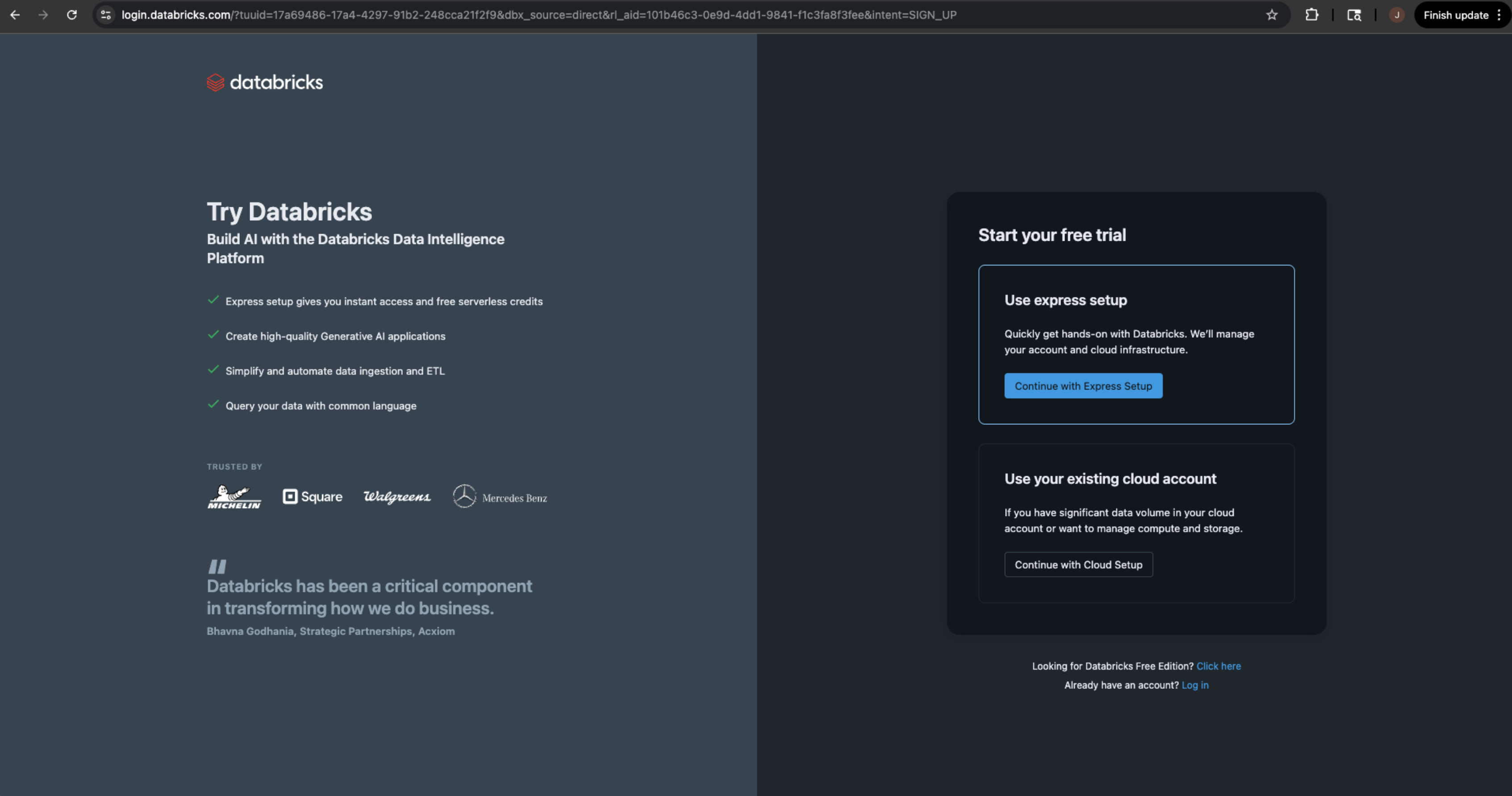
1. Select the Express Setup for a Databricks trial account form . Use an email address that is not associated with an existing Databricks account.

   

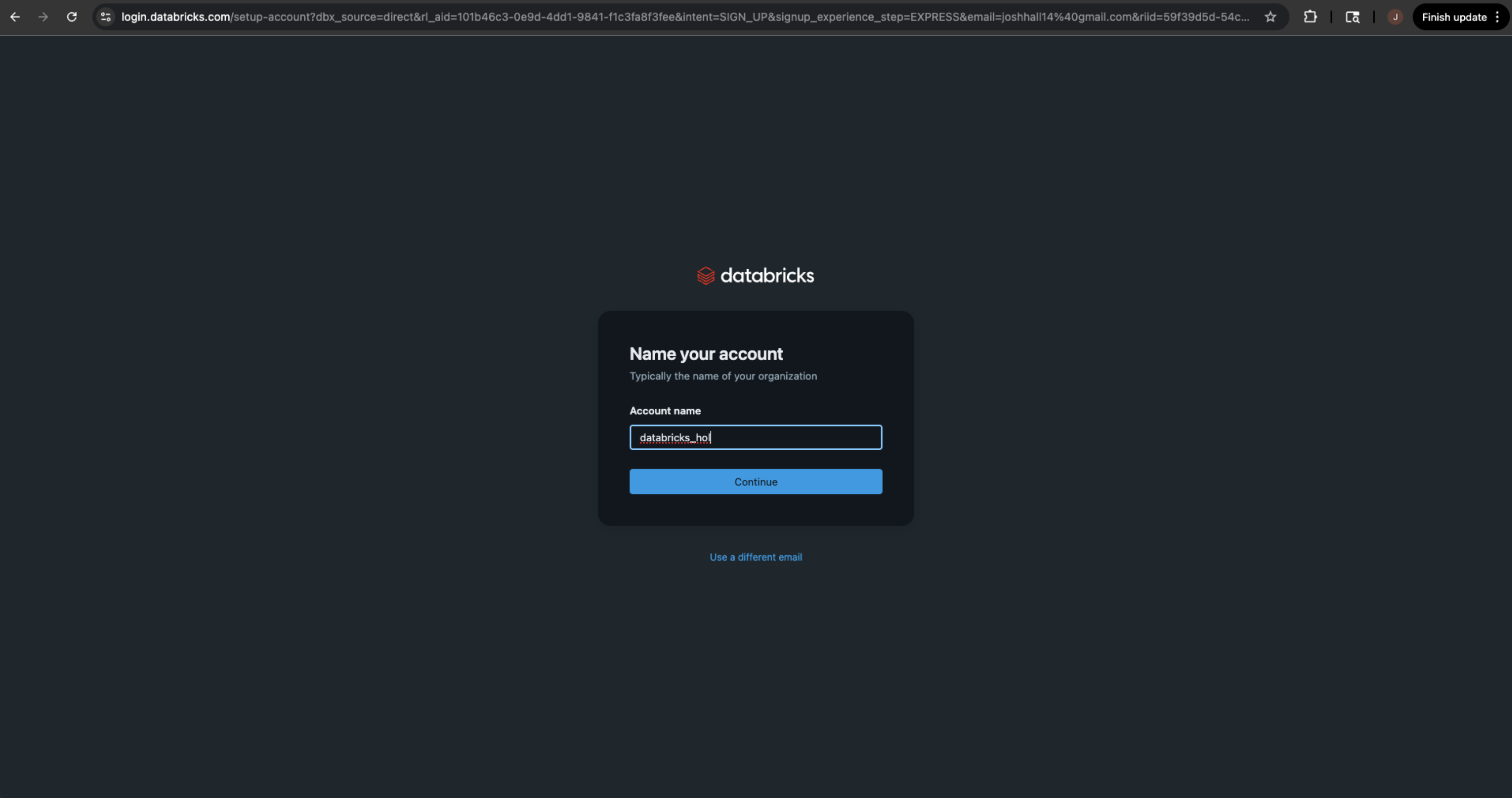
2. Give your account a meaningful name. You will have access to your Databricks trial account for 30 days. Then select the country you will be using your Databricks trial in.

   

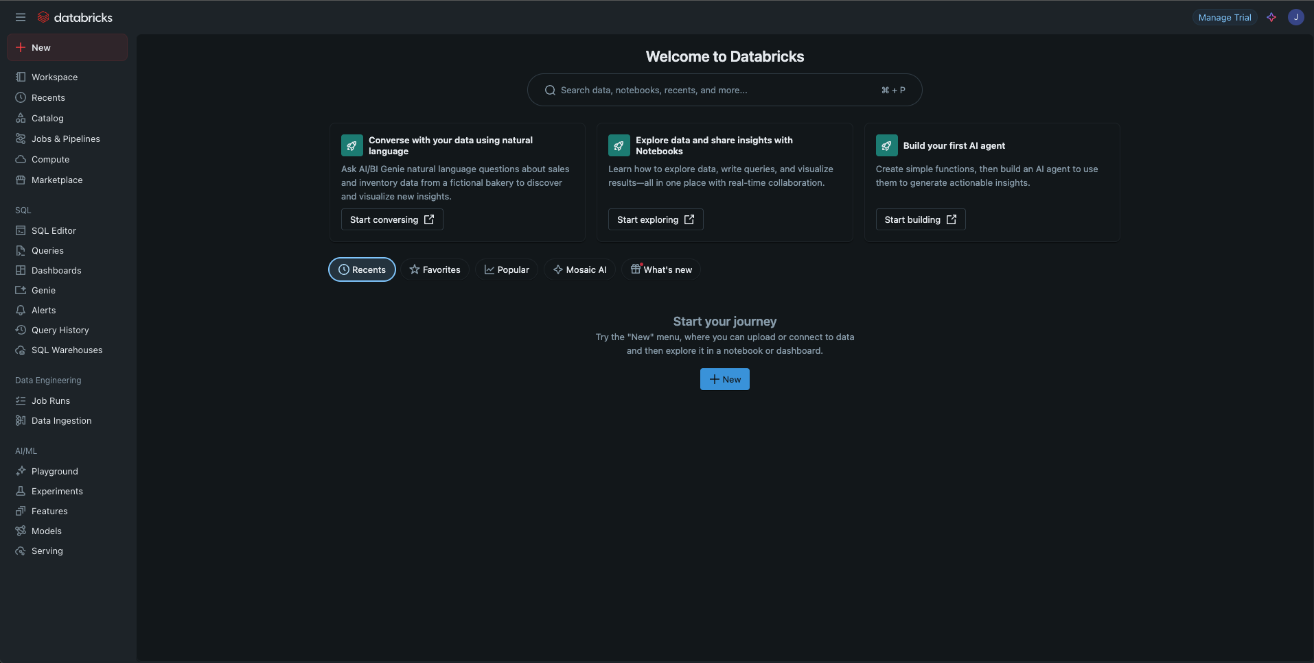
3. Once complete, Databricks will set up your account and you will land on the Databricks homepage. Your Databricks trial account is ready to go. Make sure you save the URL of your account so you can access it in the future.

   

Step 2: Create a Coalesce Trial Account

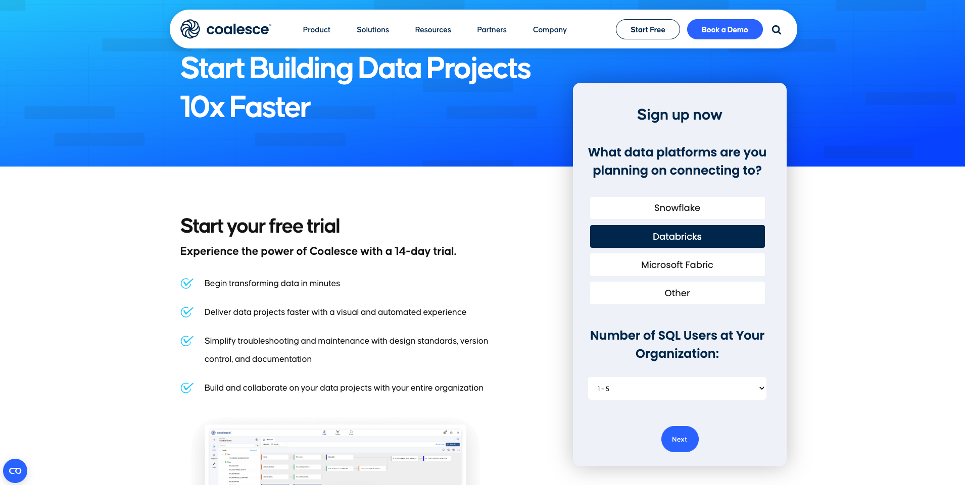
1. Next, you’ll need to sign up for a free Coalesce trial account. To do this, navigate to the Coalesce .

2. Select the data platform you want to connect to, for this lab, select Databricks. Then, select the number of SQL users you want to support. Since you’re likely doing this lab on your own, select 1-5.

   

3. Next, fill in the information to set up your trial account. If you have an existing Coalesce account, use an email that is not associated with an existing Coalesce account.

   

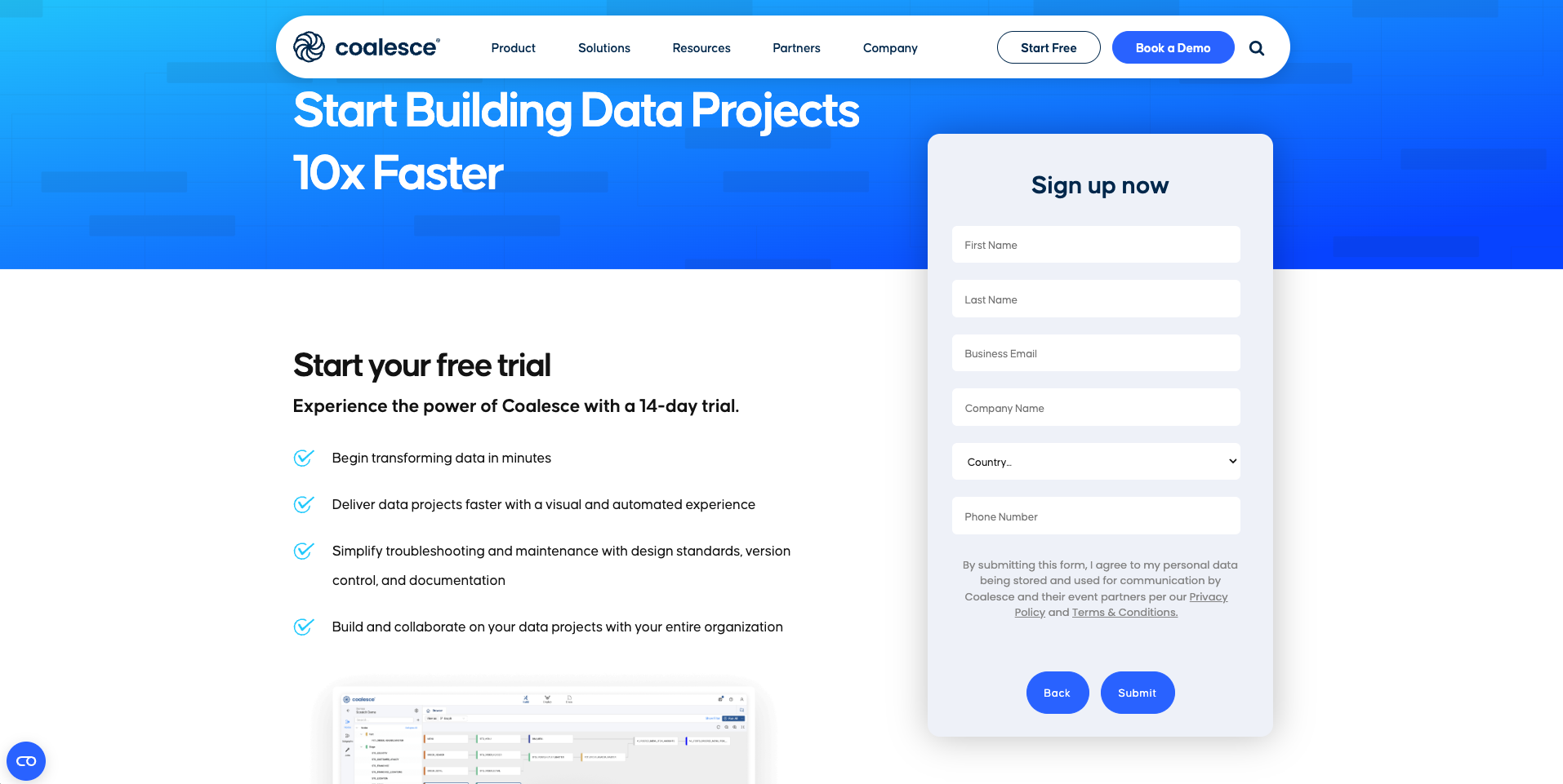
4. Select the Submit button. Within a few minutes, you will receive your trial account email, sent to the email address provided in the submission form.

   

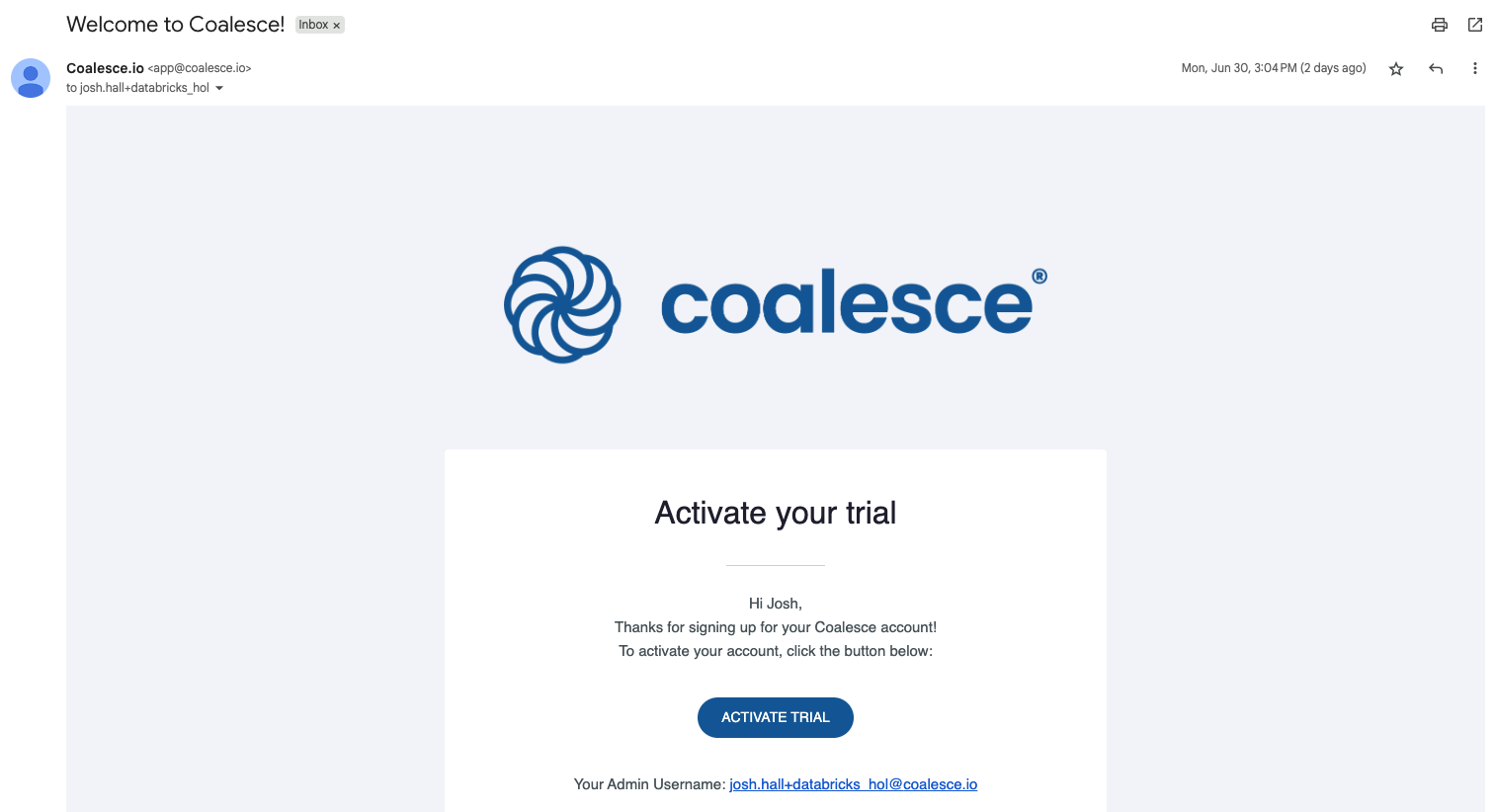
5. Click the ACTIVATE TRIAL button in the email. You will be taken to an activation page where you will fill out your account based information.

   

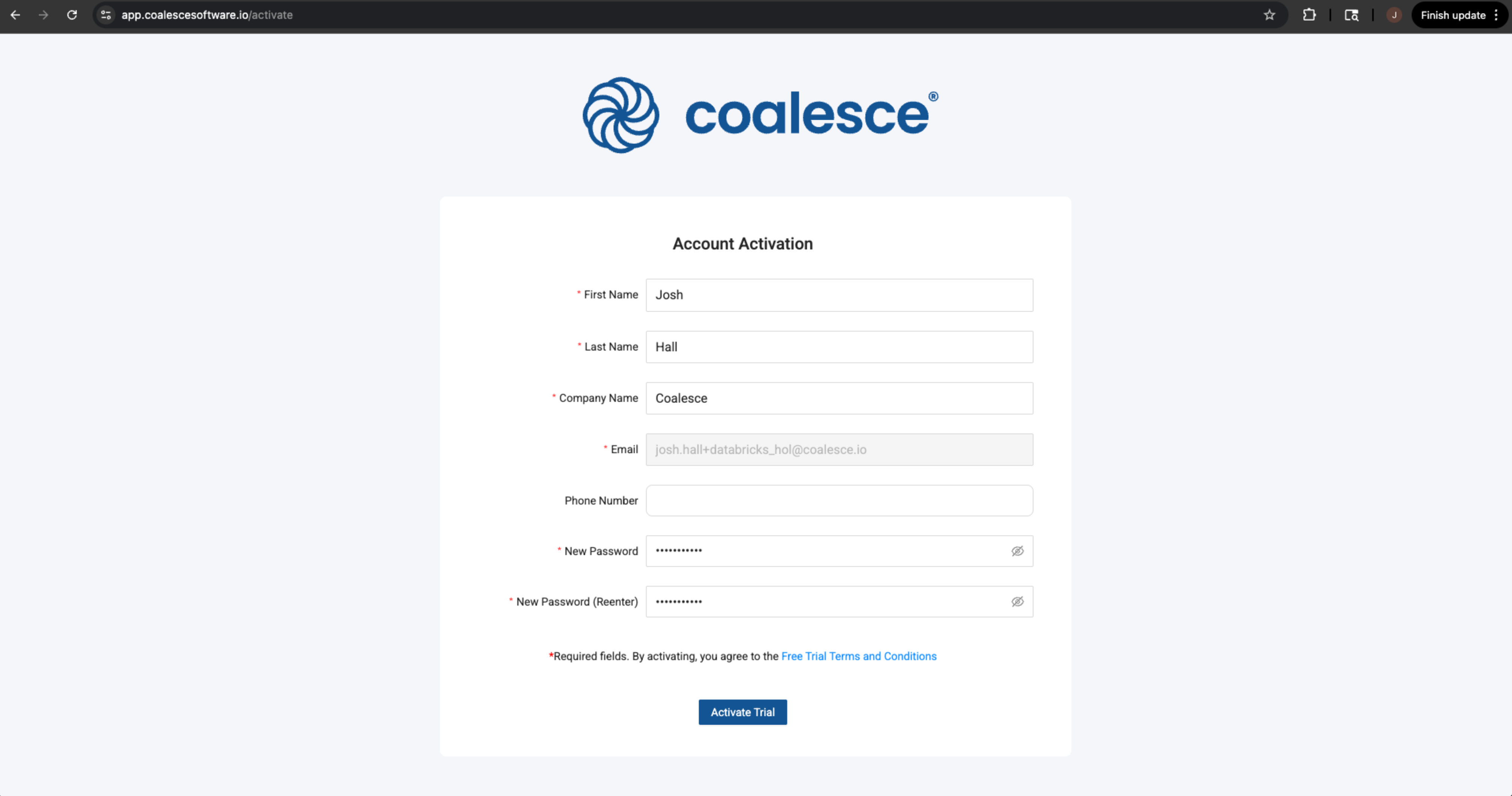
6. Select activate Trial and you will land inside of the Coalesce platform!

7. Congratulations! You’ve successfully created your Coalesce trial account.

8. Once you’ve activated your Coalesce trial account and logged in, you will land in your Projects dashboard. Projects are a useful way of organizing your development work by a specific purpose or team goal, similar to how folders help you organize documents in Google Drive.

Creating a Project in Coalesce

Now that you have a Coalesce and Databricks trial account, it’s time to connect the two together. The first step is creating a project that uses Databricks as the supported platform.

1. In the upper left corner of the projects page, select the plus + button to create a new project.

   

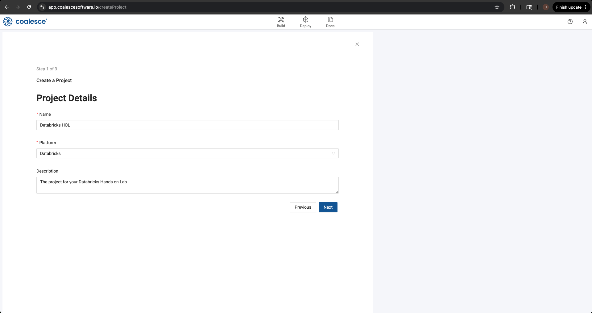
2. Give your project a name, select Databricks as your platform, and give an optional description.

   

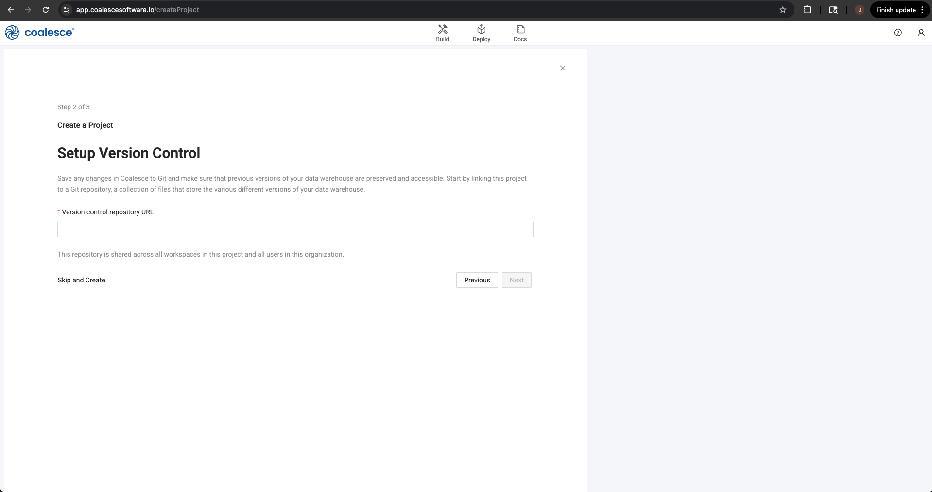
3. Select the Next button, where you’ll be asked about setting up version control. Coalesce supports a variety of Version Control platforms and we recommend this for anyone using Coalesce in their job. However, as it requires additional set up, and setting up version control is not a requirement to build, we will be skipping this step. Select the Skip and Create button in the lower left corner of the modal.

   

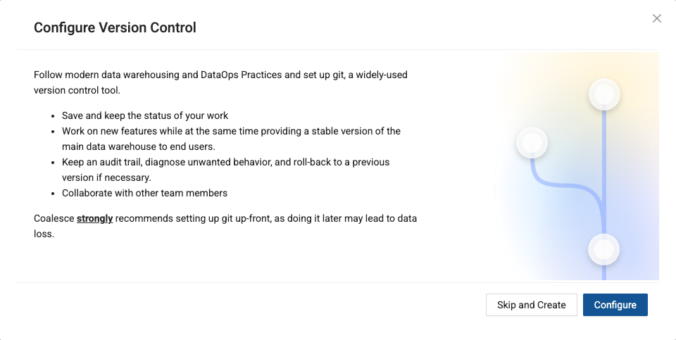
4. You’ll receive a warning message that you are about to proceed with creating a project that is not version controlled. Select Skip and Create to confirm.

   

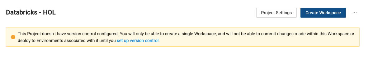
5. Congratulations, you now have a project in Coalesce that supports development on Databricks. In the next section, we’ll create a workspace that connects directly to your Databricks trial account.

Creating a Workspace

Now that you have a project created to support Databricks development, you need to create a workspace to actually build your data products. That’s what a workspace is for. Let’s create a workspace and connect it to your Databricks account.

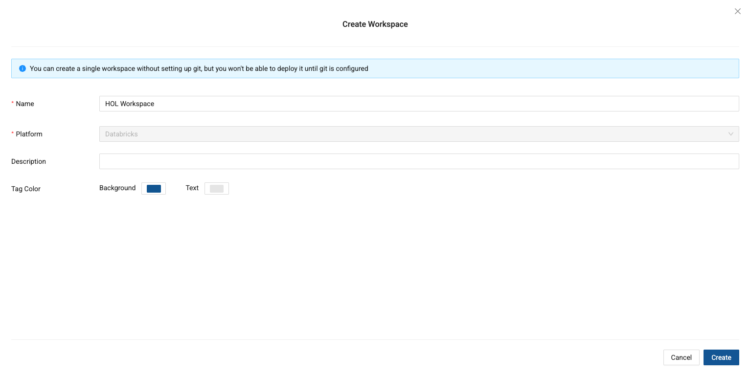
1. In your new project, select the blue Create Workspace button to create a new workspace.

   

2. Give your workspace a name and optionally provide a description.

   

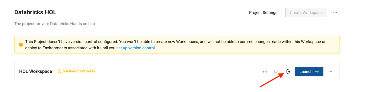
3. Now in the projects page, you should see a new workspace! Click the gear icon next to the blue Launch button to configure your workspace and connect it to Databricks.

   

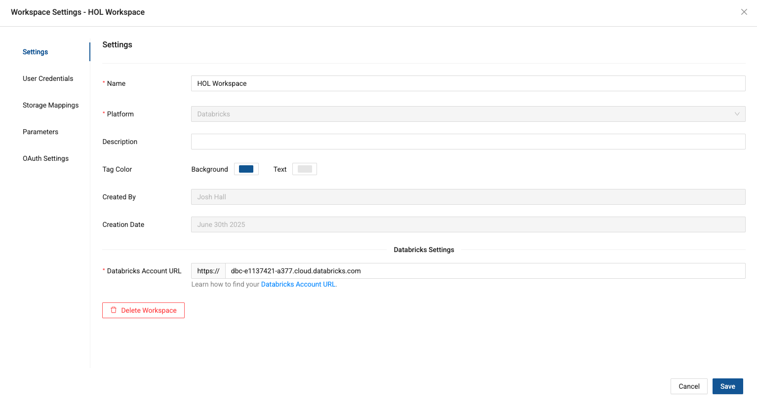
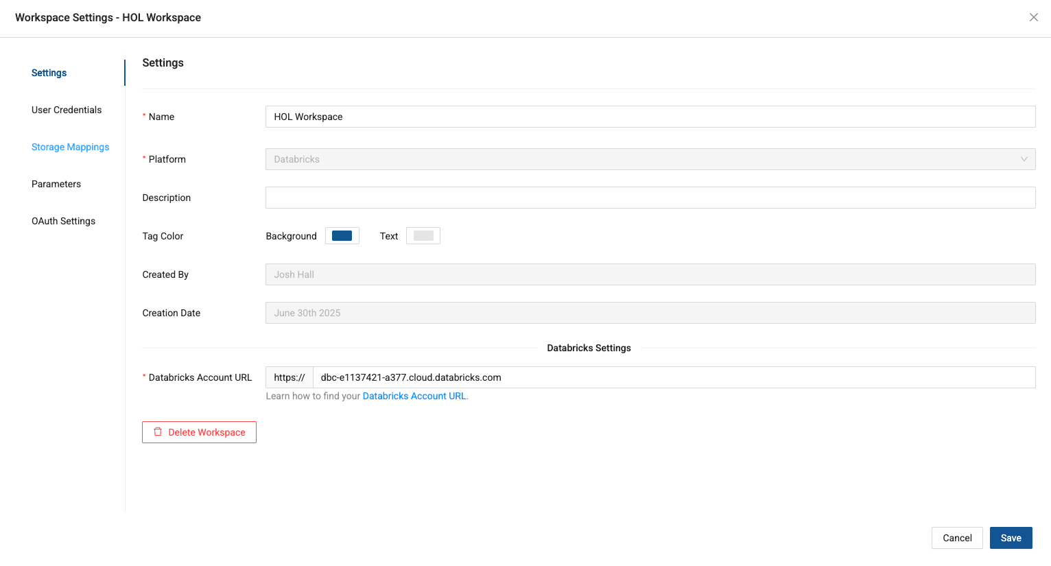
4. This will open the workspace settings. The first thing we need to do is provide the Databricks account URL we are connecting to.

   

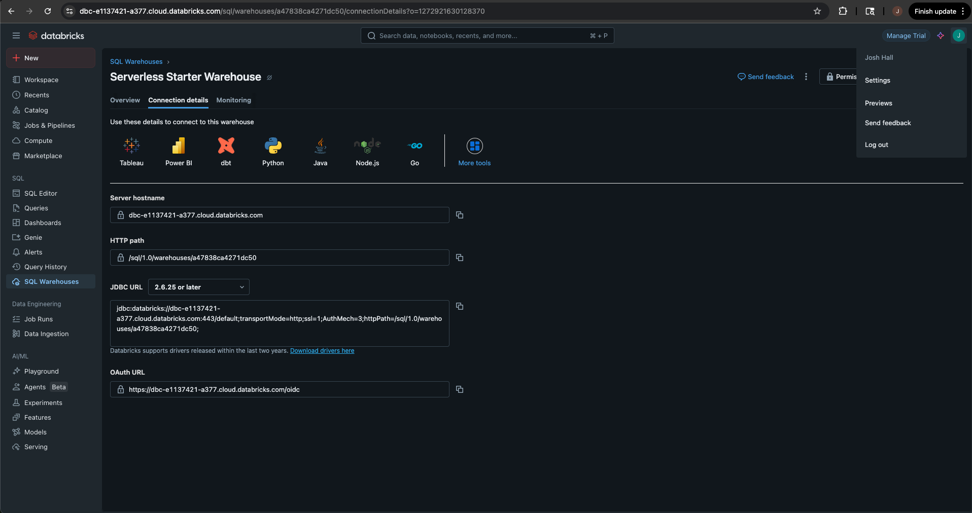
5. To do this, navigate to your Databricks trial and select SQL Warehouses.

   

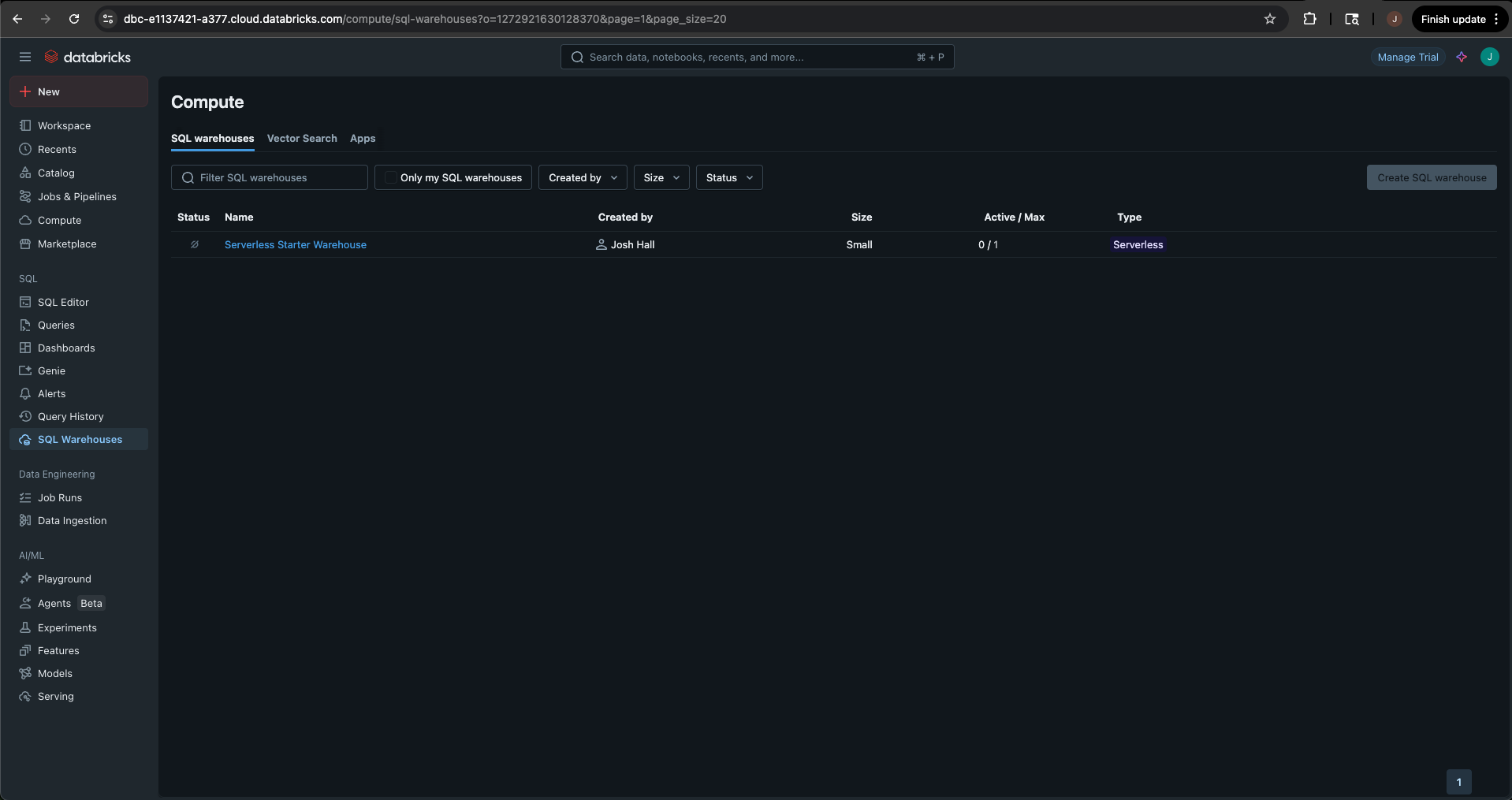
6. Select the warehouse listed (Serverless Starter Warehouse) and select the Connection details tab. You will need to copy the Server Hostname to your clipboard. You can do this by selecting the copy icon next to the Server Hostname string.

   

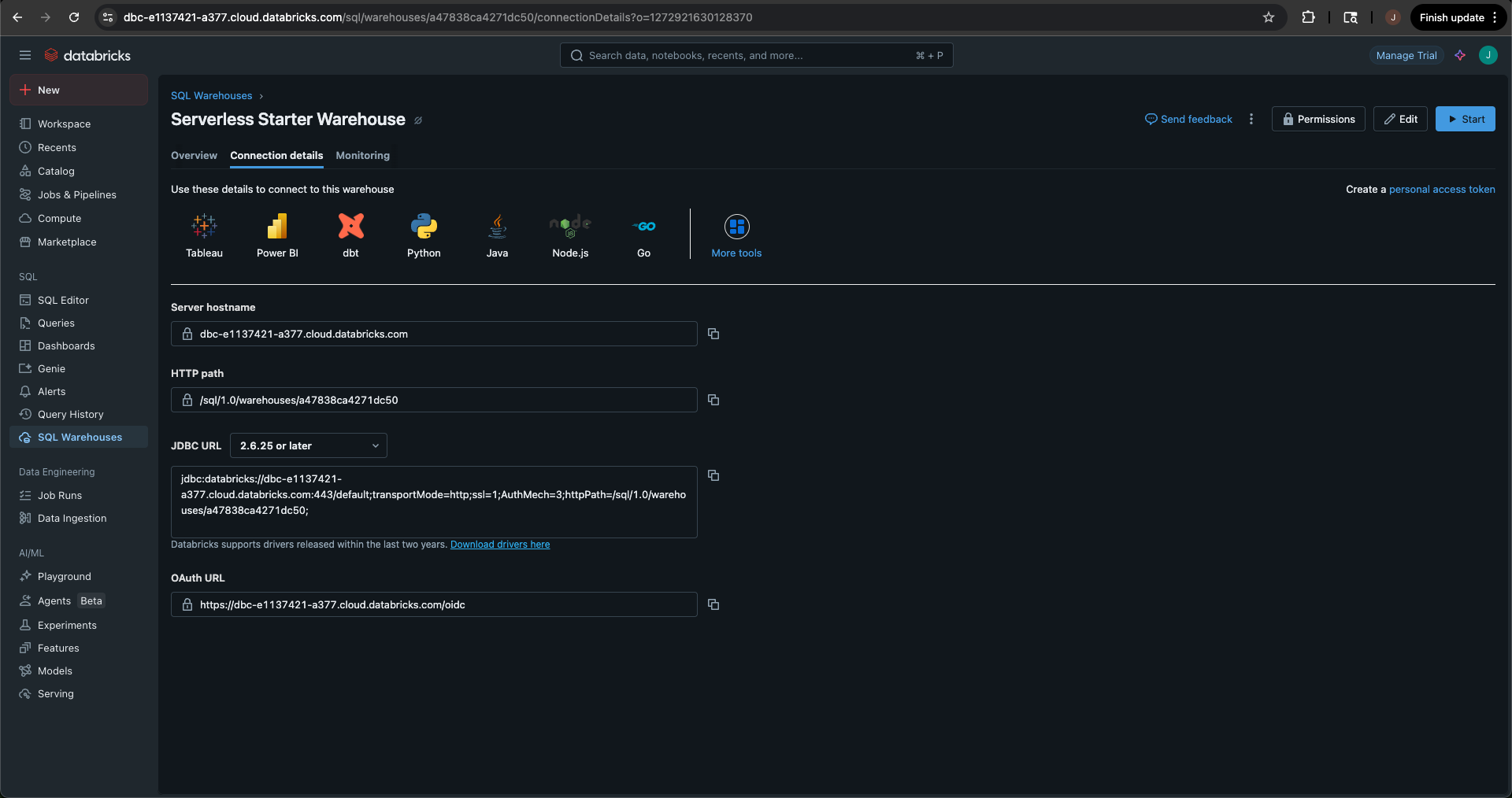
7. Return to Coalesce and provide the string in the Databricks account URL field. Once done, make sure to select Save to save the changes to your workspace.

   

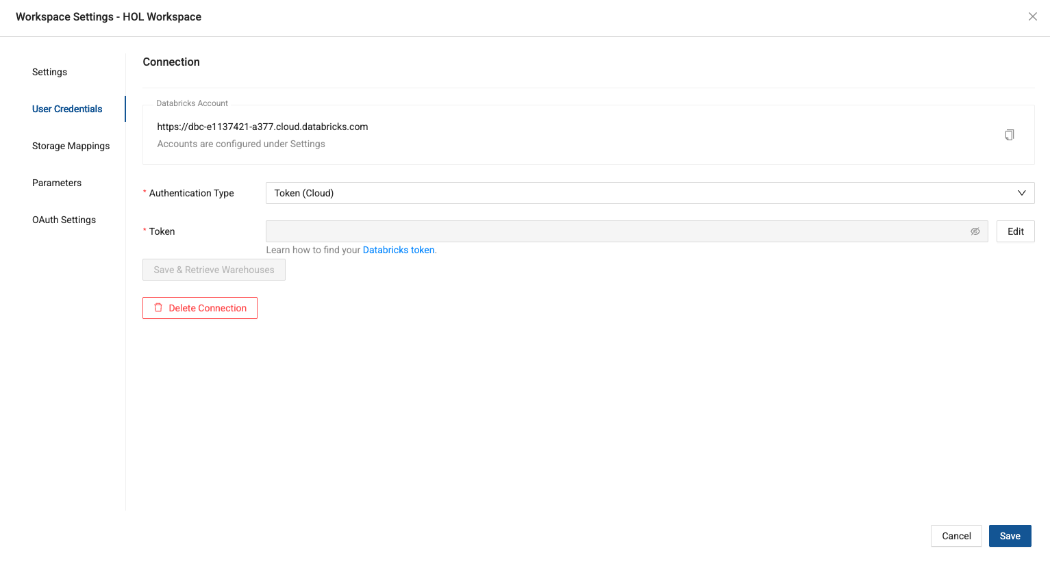
8. Next, navigate to the User Credentials tab in the workspace modal. This is where we will provide the authentication to our Databricks trial account.

   

9. The default authentication type is Token (Cloud), which is what we will be using. Navigate back to your Databricks trial account one last time. This time, select your personal settings in the upper right corner of the screen and select Settings.

   

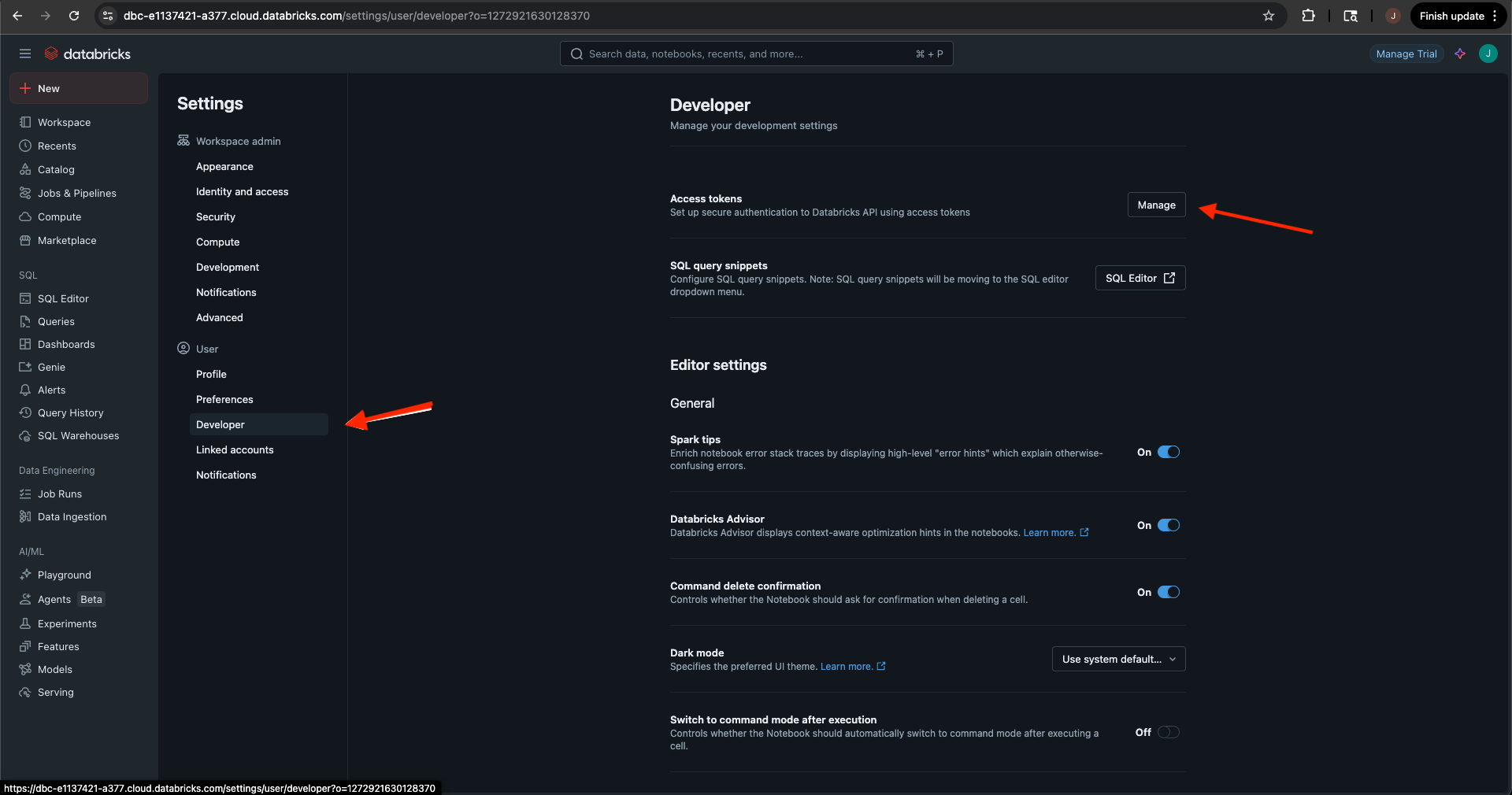
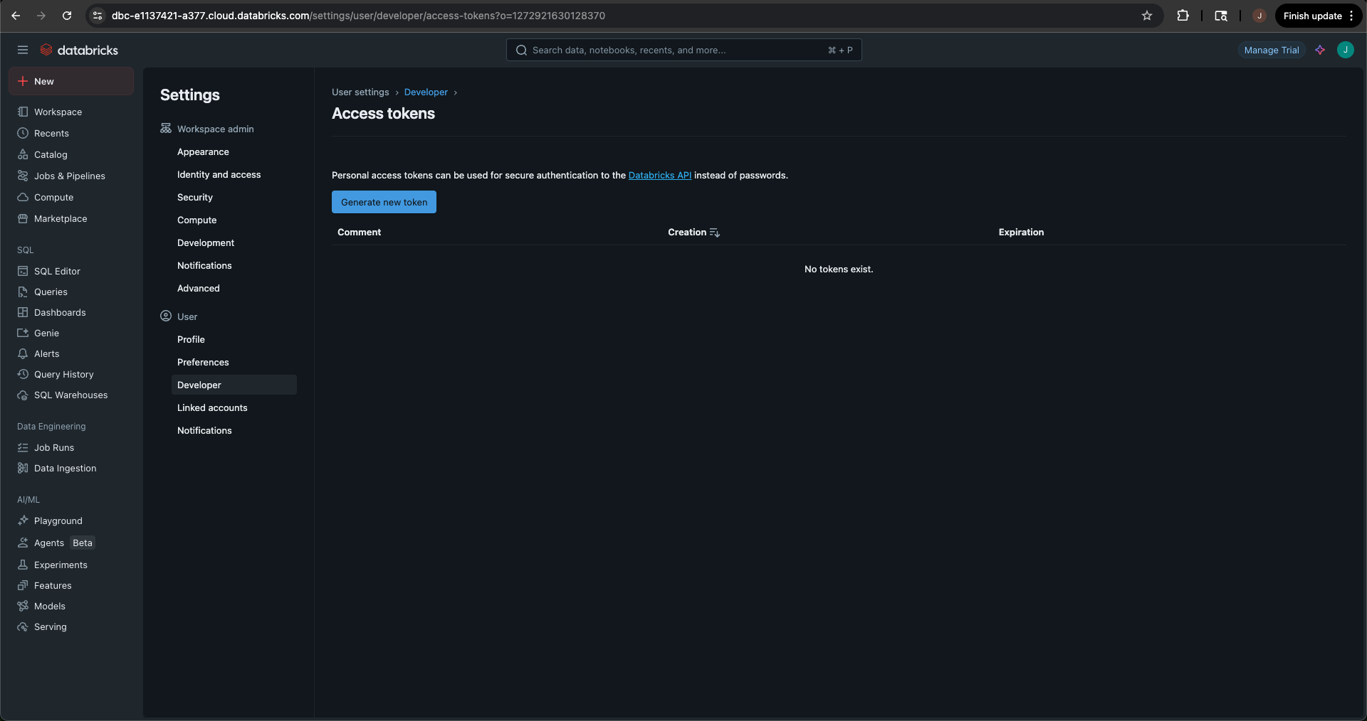
10. Within the settings, select Developer from the User men and then select Manage next to Access tokens.

    

11. On the Access tokens page, select the blue Generate new token button.

    

12. Give the token a comment and set the lifetime. You can leave the default at 90 days.

    

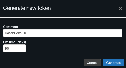
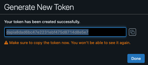
13. Select the blue Generate button. This will display your new access token. Be sure to copy this to your clipboard so we can paste it into Coalesce.

    

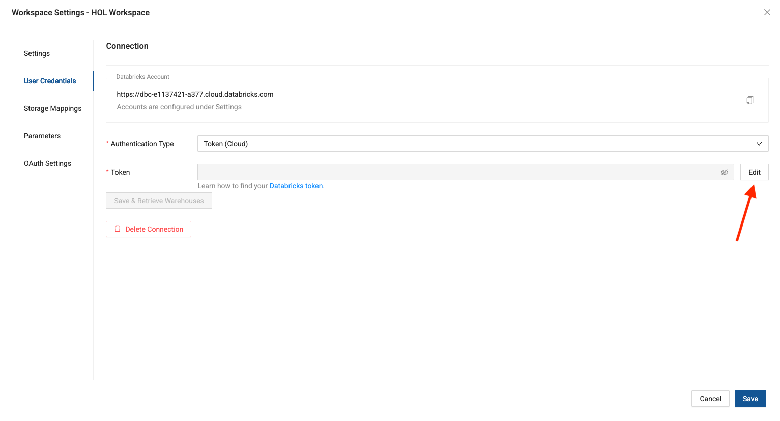
14. Navigate back to Coalesce. Select the edit button next to the token field and paste in the access token you created in Databricks.

    

15. You should now have the ability to save & retrieve the SQL warehouse available in your Databricks account, to use to run your Coalesce objects.

    

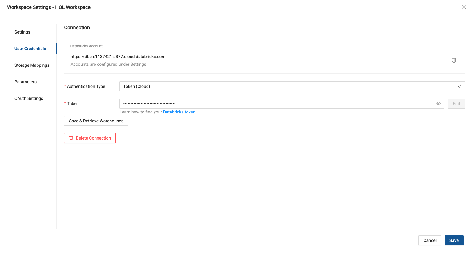
16. Select the Serverless start warehouse available and then select the blue save button to save all of your changes.

    

17. You have now connected your Coalesce trial account to your Databricks trial account and can start building your data products.

Navigating the Coalesce User Interface

Let's get familiar with Coalesce by walking through the basic components of the user interface.

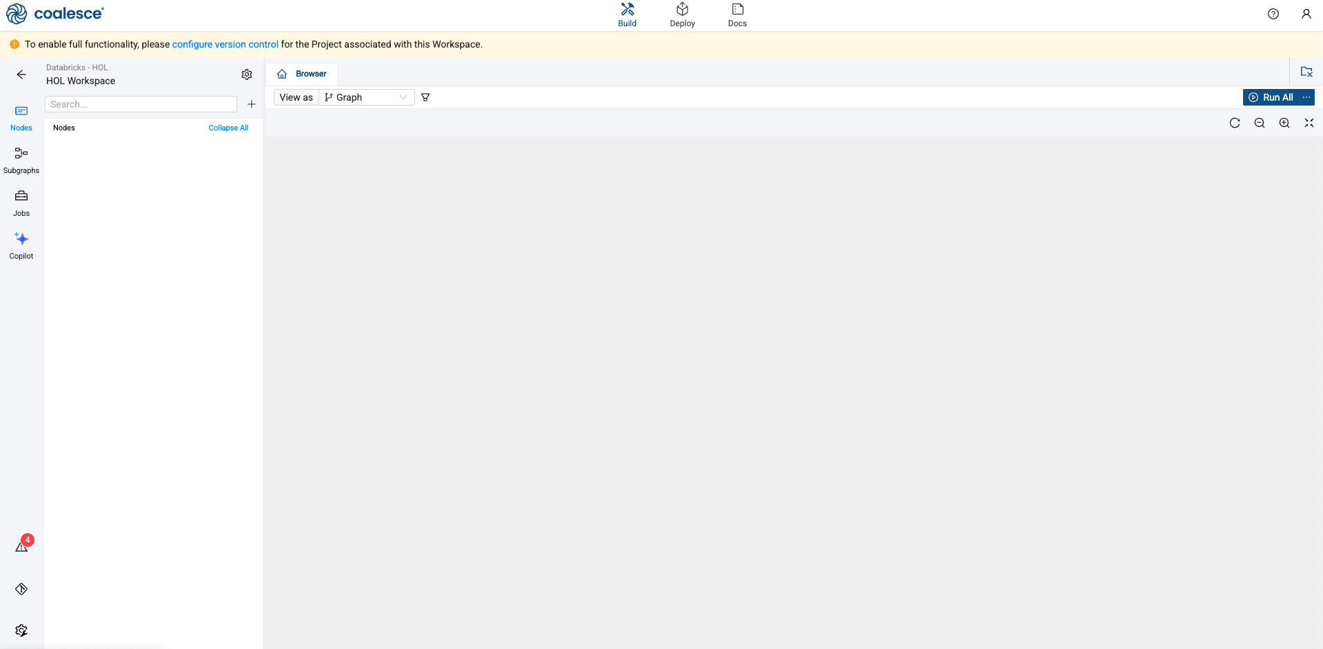
1. Upon launching your Development Workspace, you’ll be taken to the Build Interface of the Coalesce UI. The Build Interface is where you can create, modify and publish nodes that will transform your data.

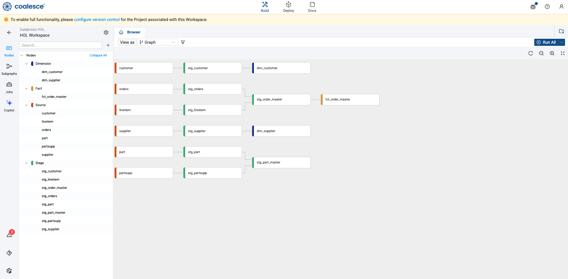
2. Nodes are visual representations of objects in Databricks that can be arranged to create a Directed Acyclic Graph (DAG or Graph). A DAG is a conceptual representation of the nodes within your data pipeline and their relationships to and dependencies on each other.

3. In the Browser tab of the Build interface, you can visualize your node graph using the Graph, Node Grid, and Column Grid views. In the upper right hand corner, there is a person-shaped icon where you can manage your account and user settings.

   

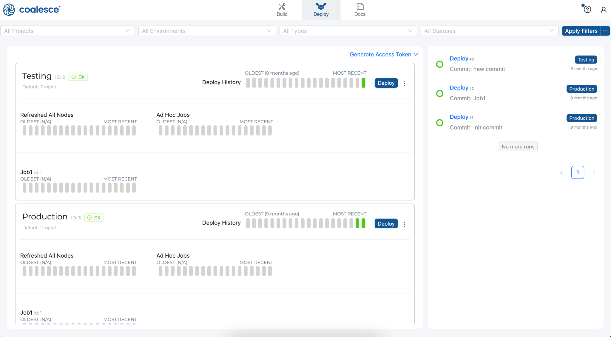
4. Next to the Build interface is the Deploy interface. This is where you will push your pipeline to other environments such as Testing or Production. Like the Browser tab, this area is currently empty but will populate as we will build out Nodes and our Graph in subsequent steps of this lab.

   

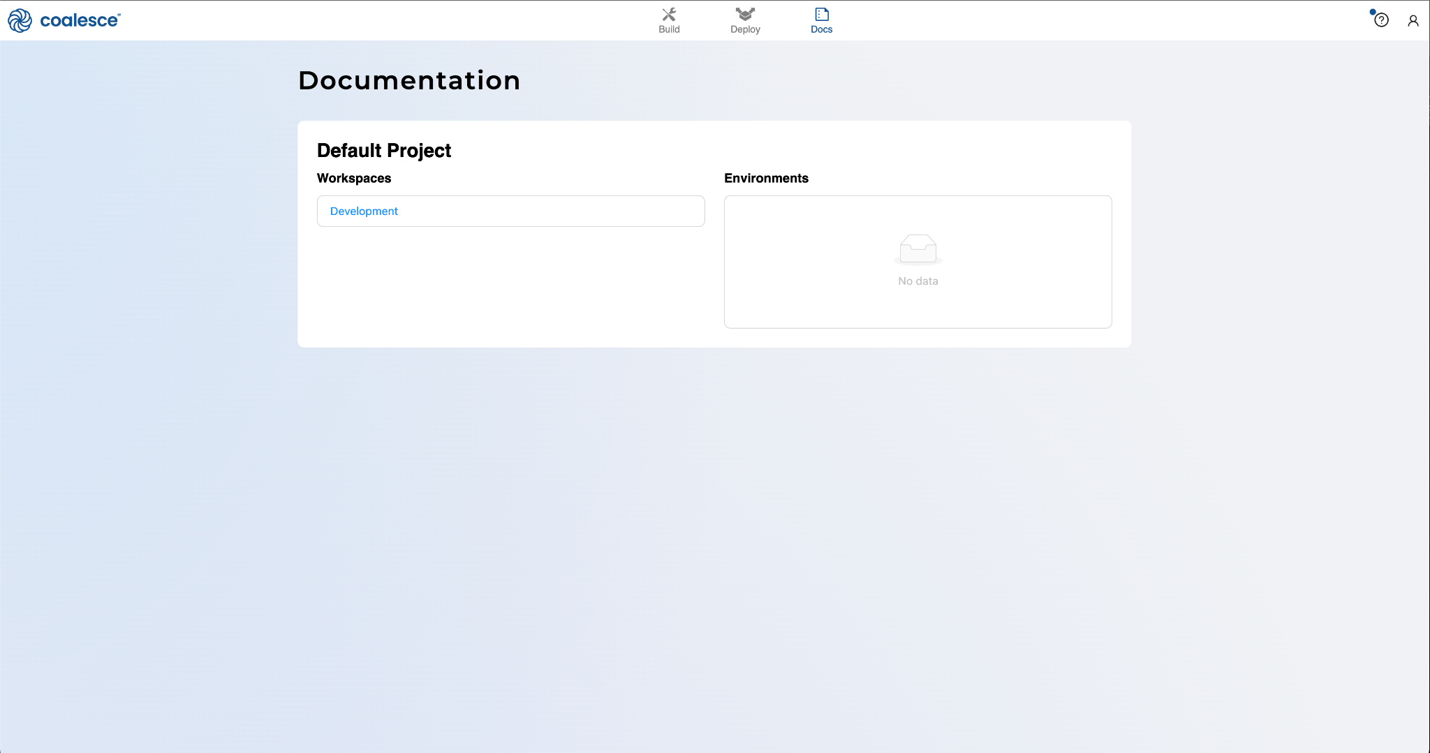
5. Next to the Deploy interface is the Docs interface. Documentation is an essential step in building a sustainable data architecture, but is sometimes put aside to focus on development work to meet deadlines. To help with this, Coalesce automatically generates and updates documentation as you work.

   

Adding Storage Locations

Storage locations are containers or pointers that allow you to designate which catalog and schema you want to represent within the Coalesce UI. We will add three storage locations in this lab.

1. To add a storage location, navigate to the build settings in the lower left corner of the screen.

   

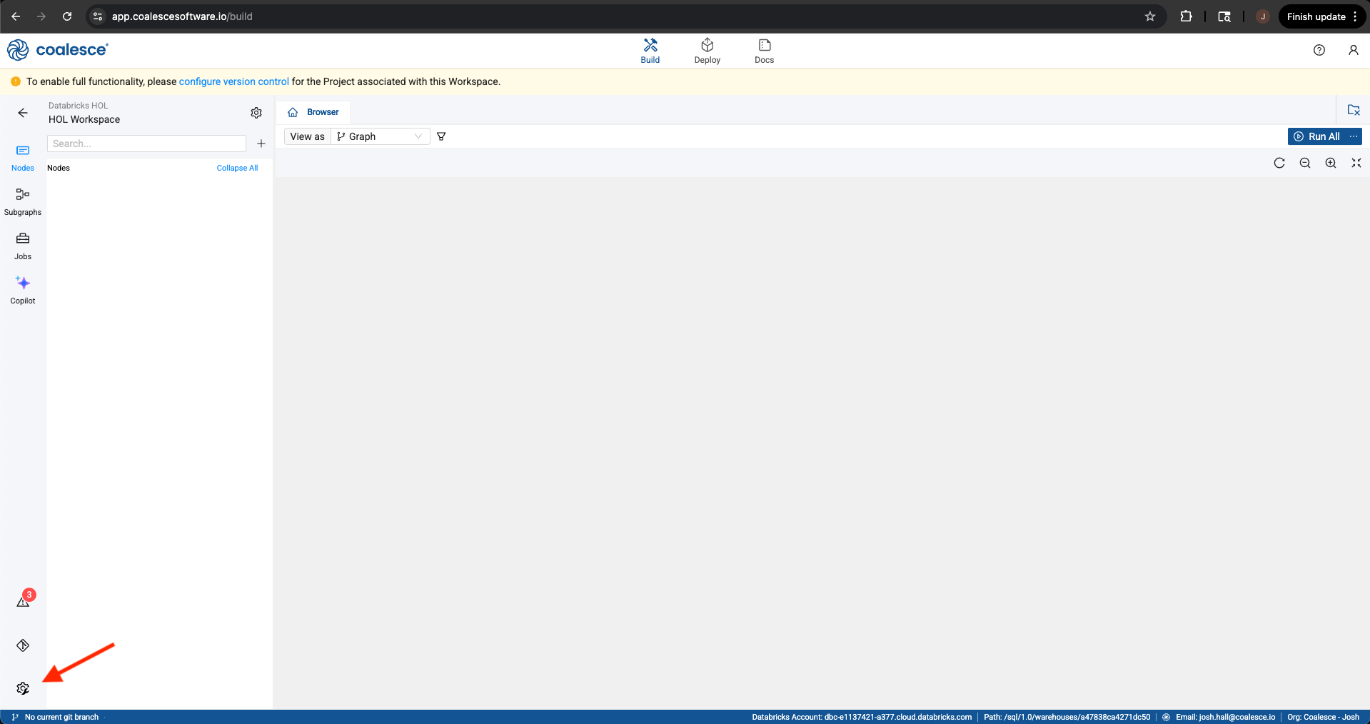
2. Within the build settings, navigate to Storage Locations.

   

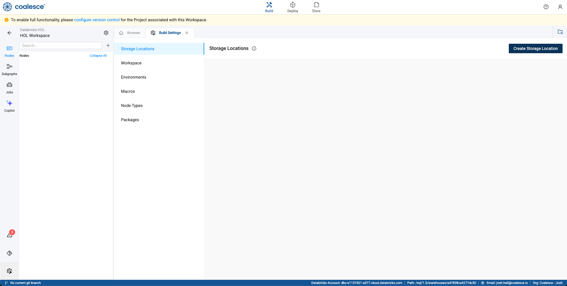
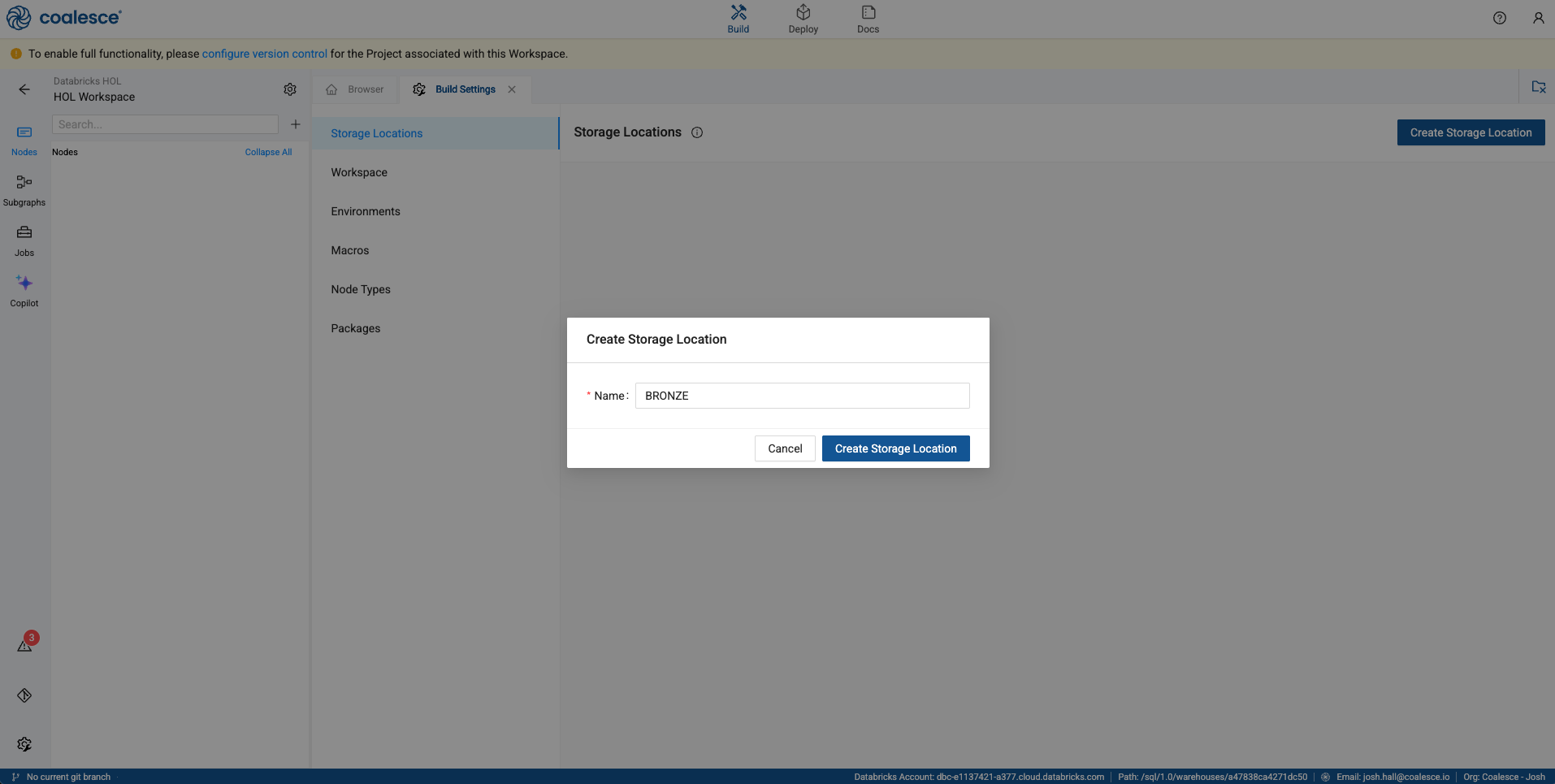
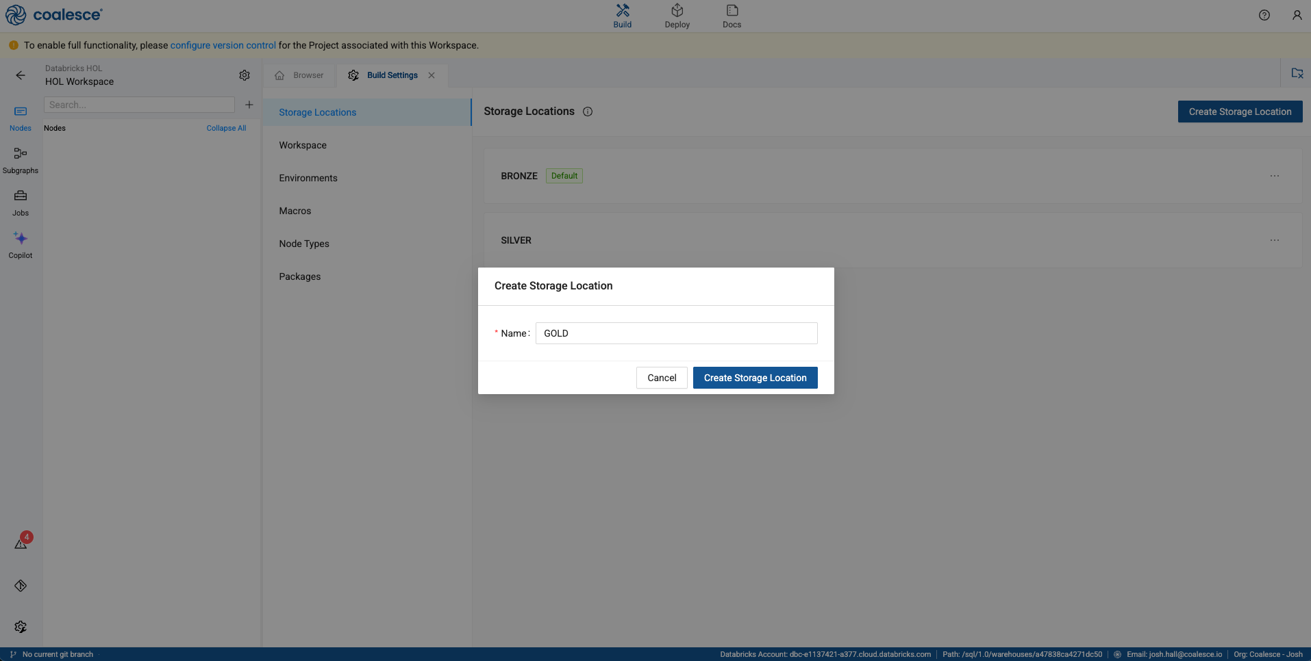
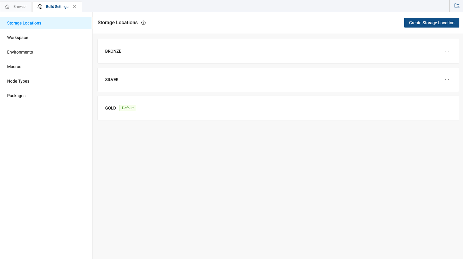
3. Select the Create Storage Location button in the upper right corner of the screen. The first storage location we’ll create is called BRONZE. In the text box, type in BRONZE and select the Create Storage Location button.

   

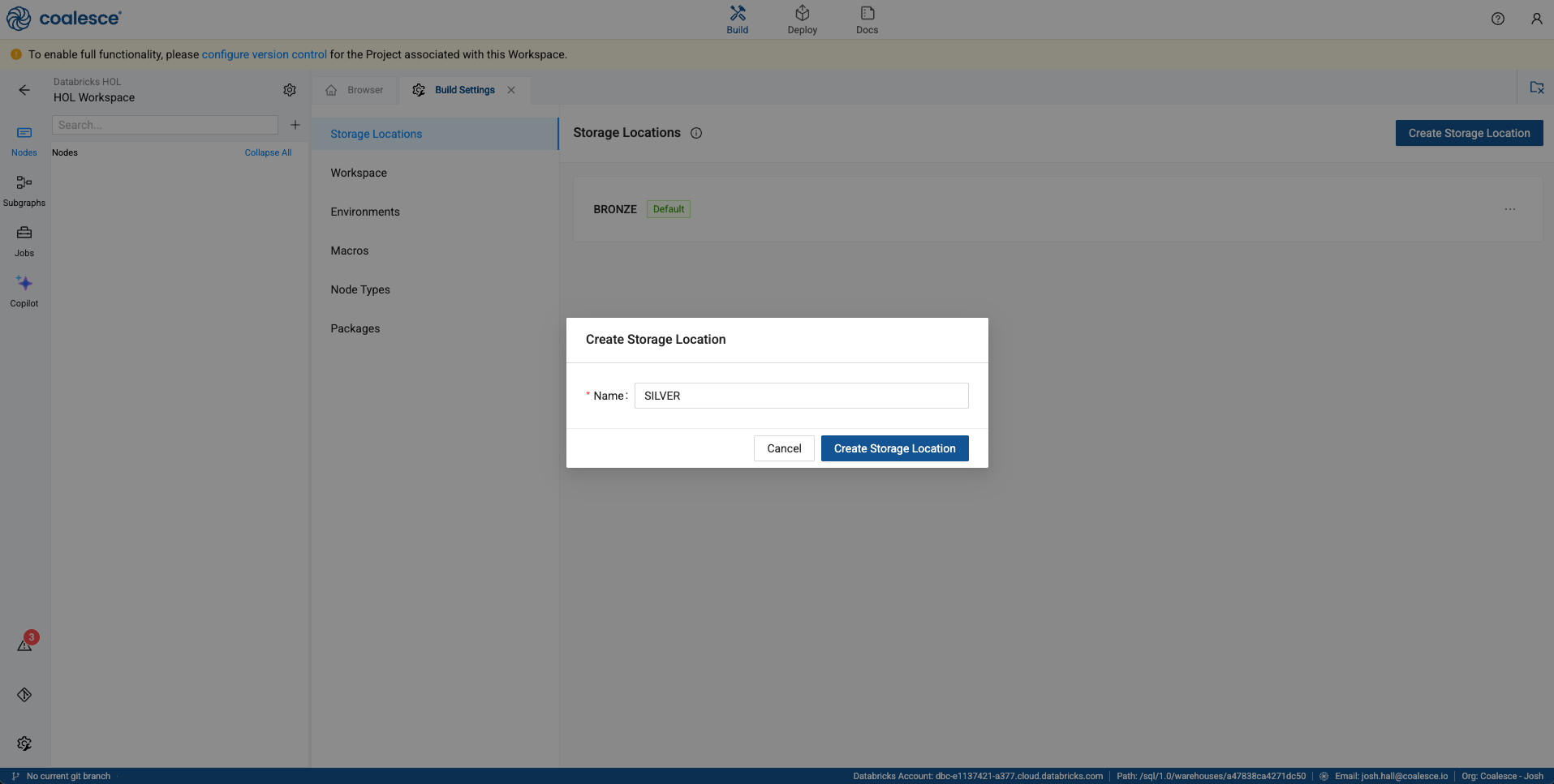
4. We’ll follow this same process to create our Silver layer.

   

5. And finally, we’ll create the gold layer.

   

6. In the storage location menu page, select the ellipses next to the GOLD storage location and select Set as Default. This will make sure that, by default, all objects created in coalesce will be persisted in this location within Databricks.

   

7. Now that we’ve created storage locations, we need to point these storage locations to physical destinations within our Data bricks account. Let’s do that next!

Configuring Storage Mappings

In order to use any data in your Databricks account, you need to point your storage locations to physical destinations within Databricks. We call these Storage Mappings in Coalesce. Let’s configure these now, at the end of which, we can begin building our data pipelines!

1. Navigate back to the workspace settings, the same place where we configured the connection to your Databricks account.

   

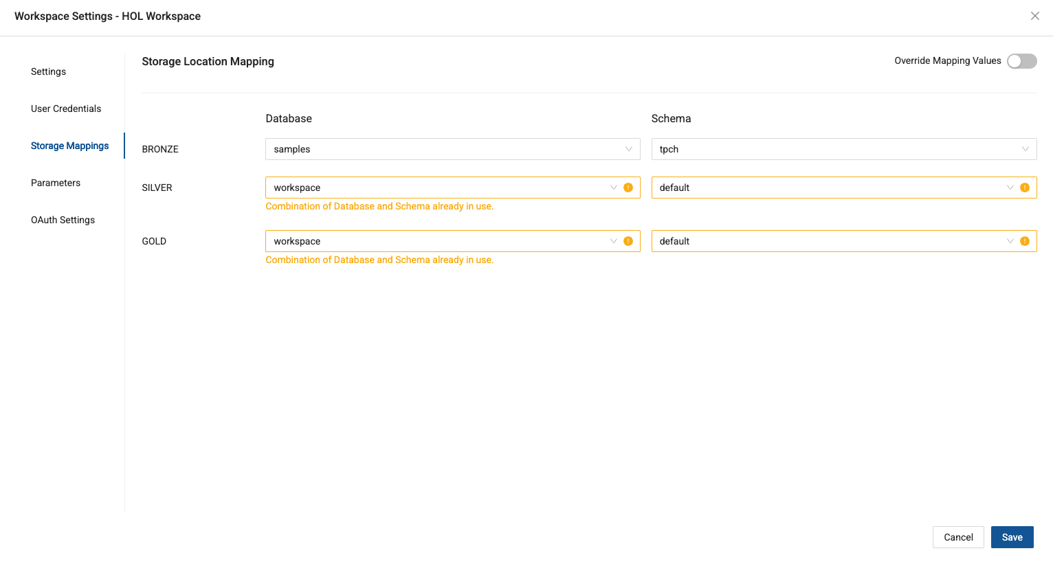
2. Navigate to the Storage Mapping menu item and you’ll map your Storage Locations with the following Catalogs and Schemas:

   • BRONZE -> samples -> tpch
   • SILVER -> workspace -> default
   • GOLD -> workspace -> default

3. You’ll get a notification that both the SILVER and GOLD layers are pointing to the same catalog and schema. While this isn’t always best practice, for the sake of this lab, this is all we need.

   

4. Make sure to save the mappings you just configured!

Adding Data Sources

Now that we have access to data, let’s start to build a Graph (DAG) by adding data in the form of Source nodes.

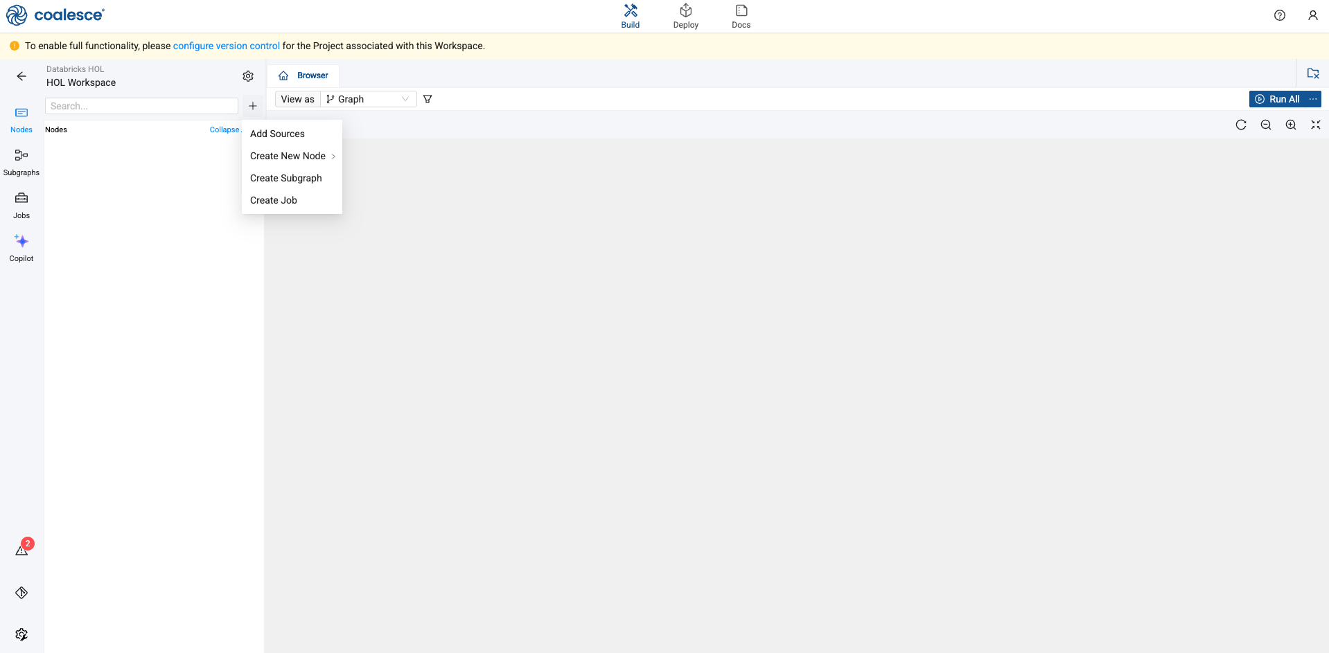
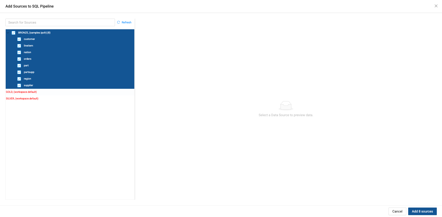
1. Start in the Build interface and click on Nodes in the left sidebar (if not already open). Click the + icon and select Add Sources.

   

2. Click to expand the tables within BRONZE storage locations and select all of the corresponding source tables underneath. Click Add Sources on the bottom right to add the sources to your pipeline.

   

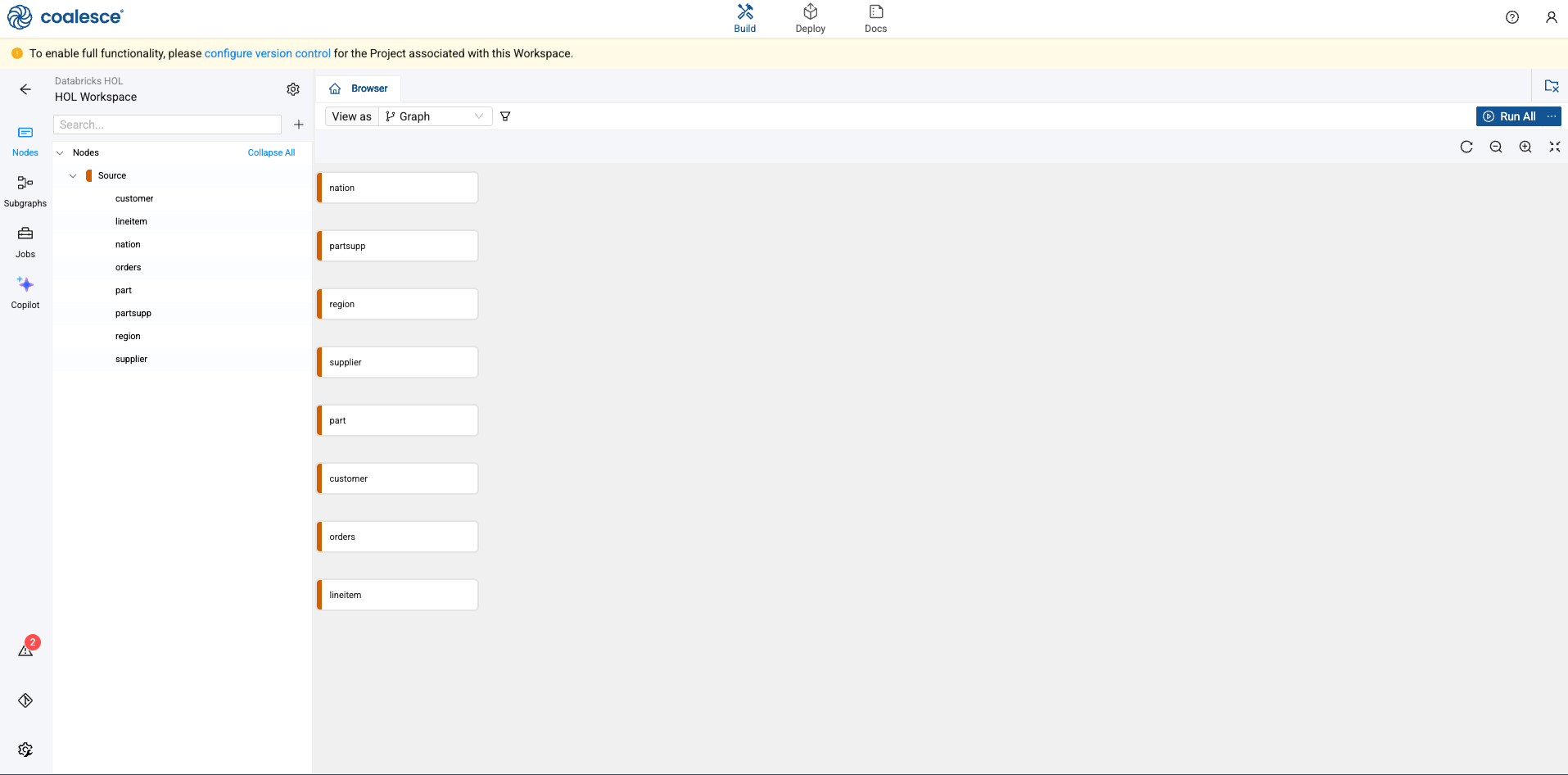
3. You'll now see your graph populated with your Source nodes. Note that they are designated in red. Each node type in Coalesce has its own color associated with it, which helps with visual organization when viewing a Graph.

   

Creating Stage Nodes

Now that you’ve added your Source nodes, let’s prepare the data by adding business logic with Stage nodes. Stage nodes represent staging tables within Databricks where transformations can be previewed and performed.

1. Let's start by adding a standardized "stage layer" for all sources.

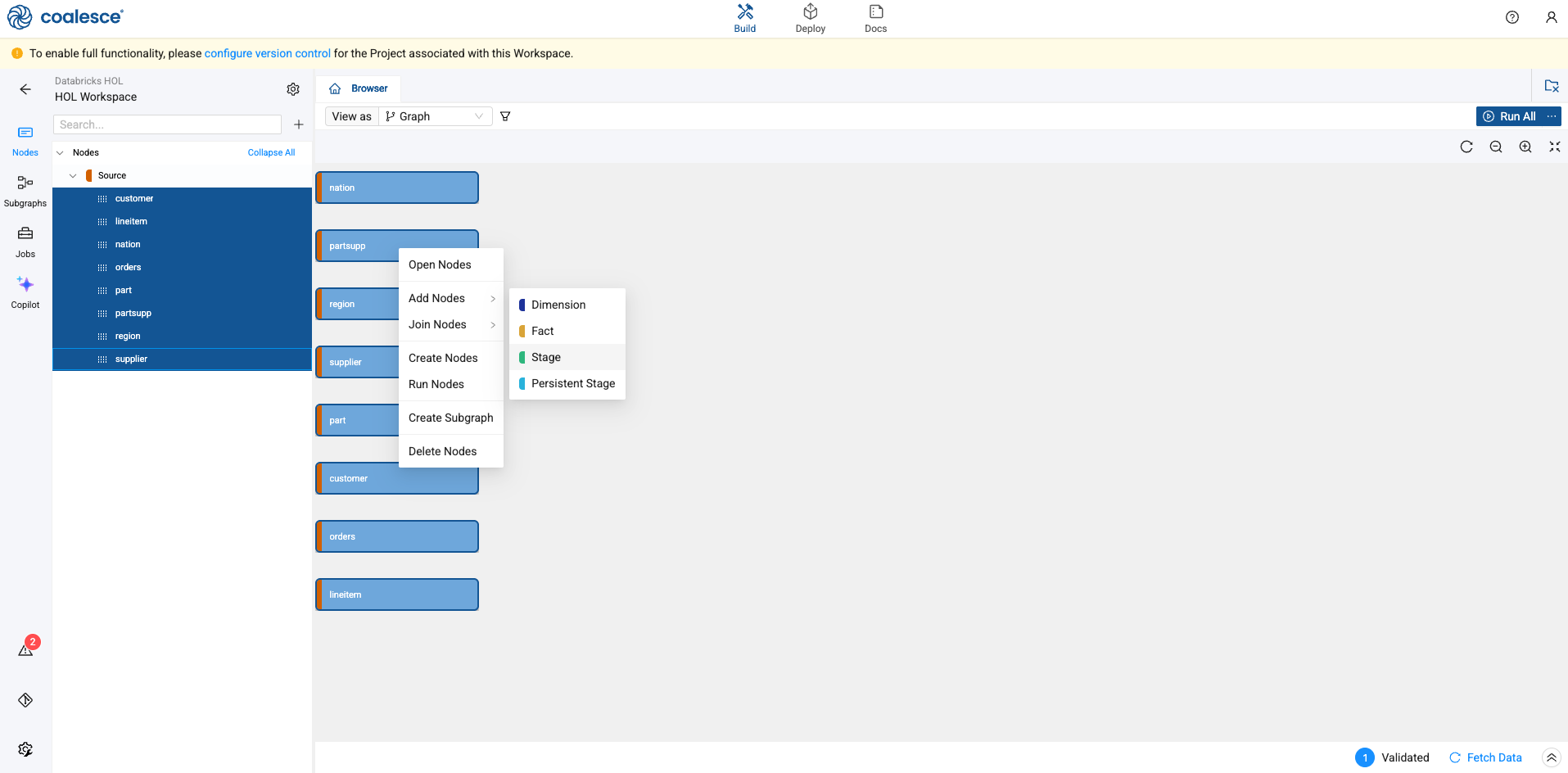
2. Press and hold the Shift key to multi-select all of your Source nodes. Then right click and select Add Node > Stage from the drop down menu.

   

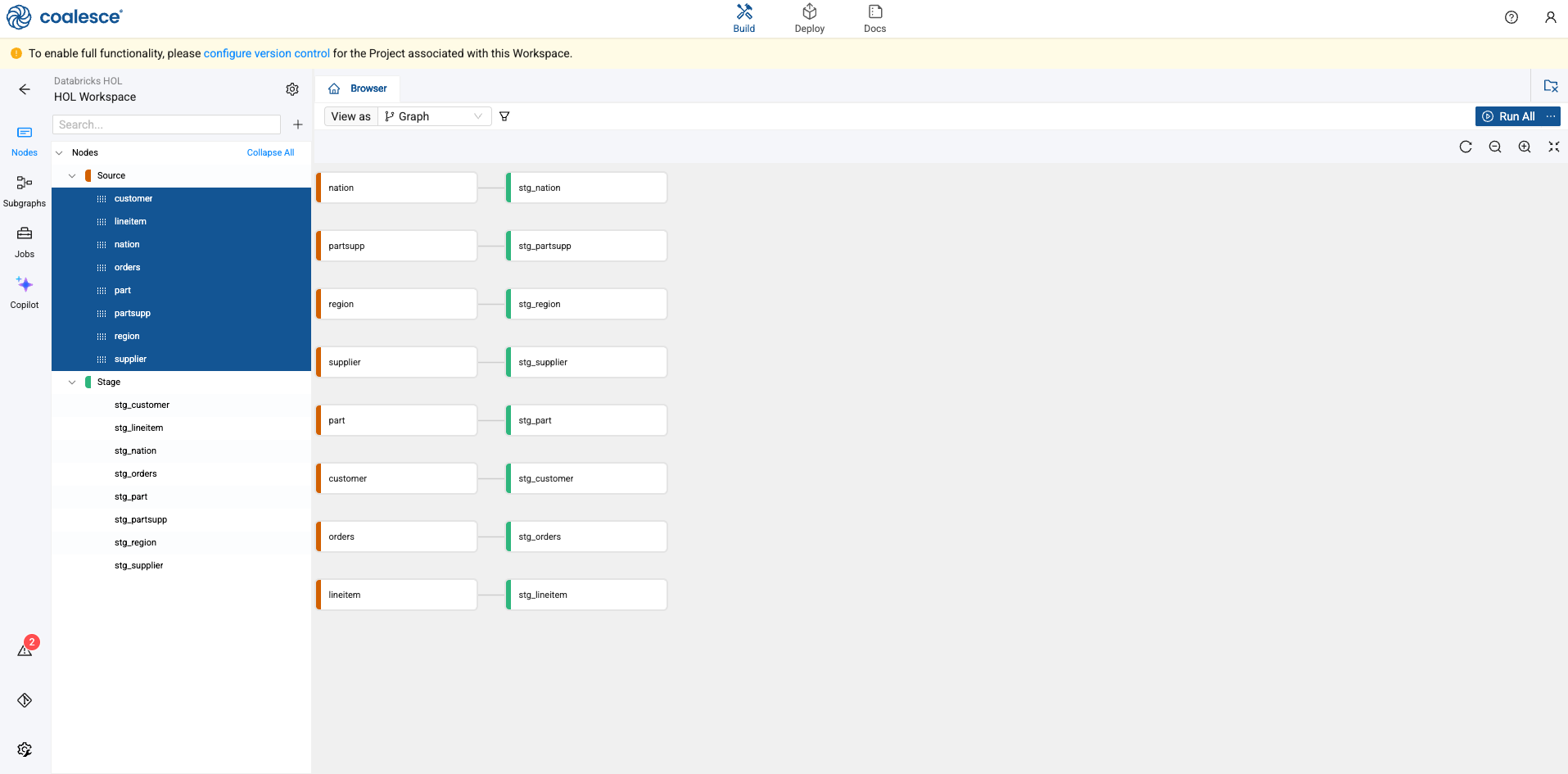
3. You will now see that all of your Source nodes have corresponding Stage tables associated with them.

   

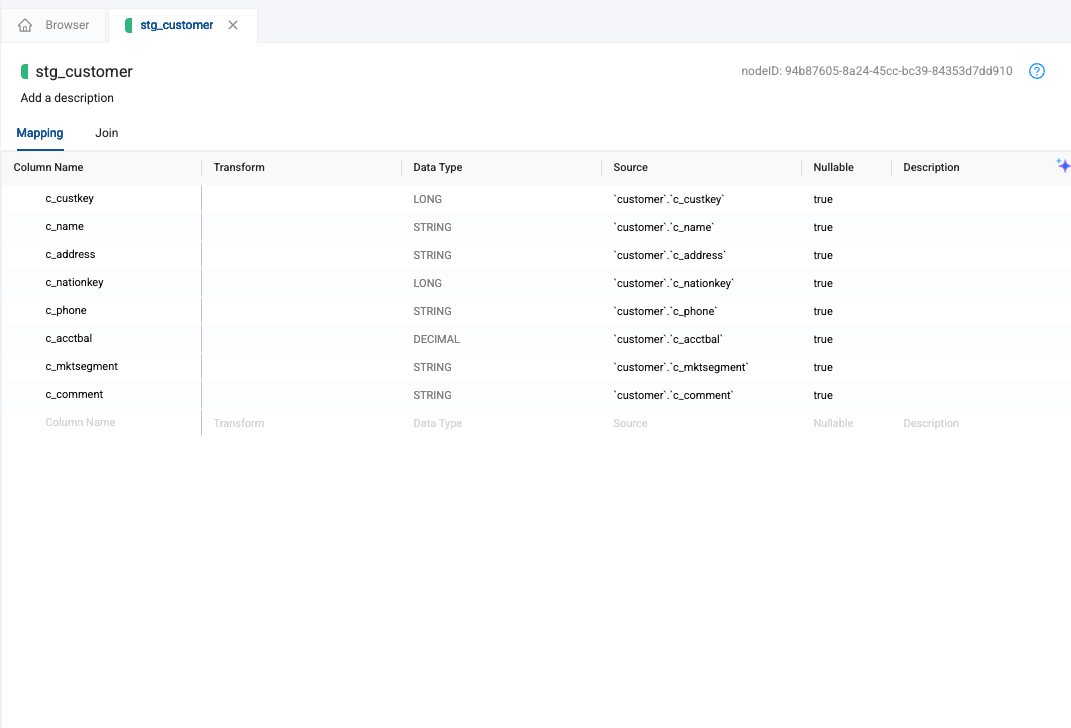
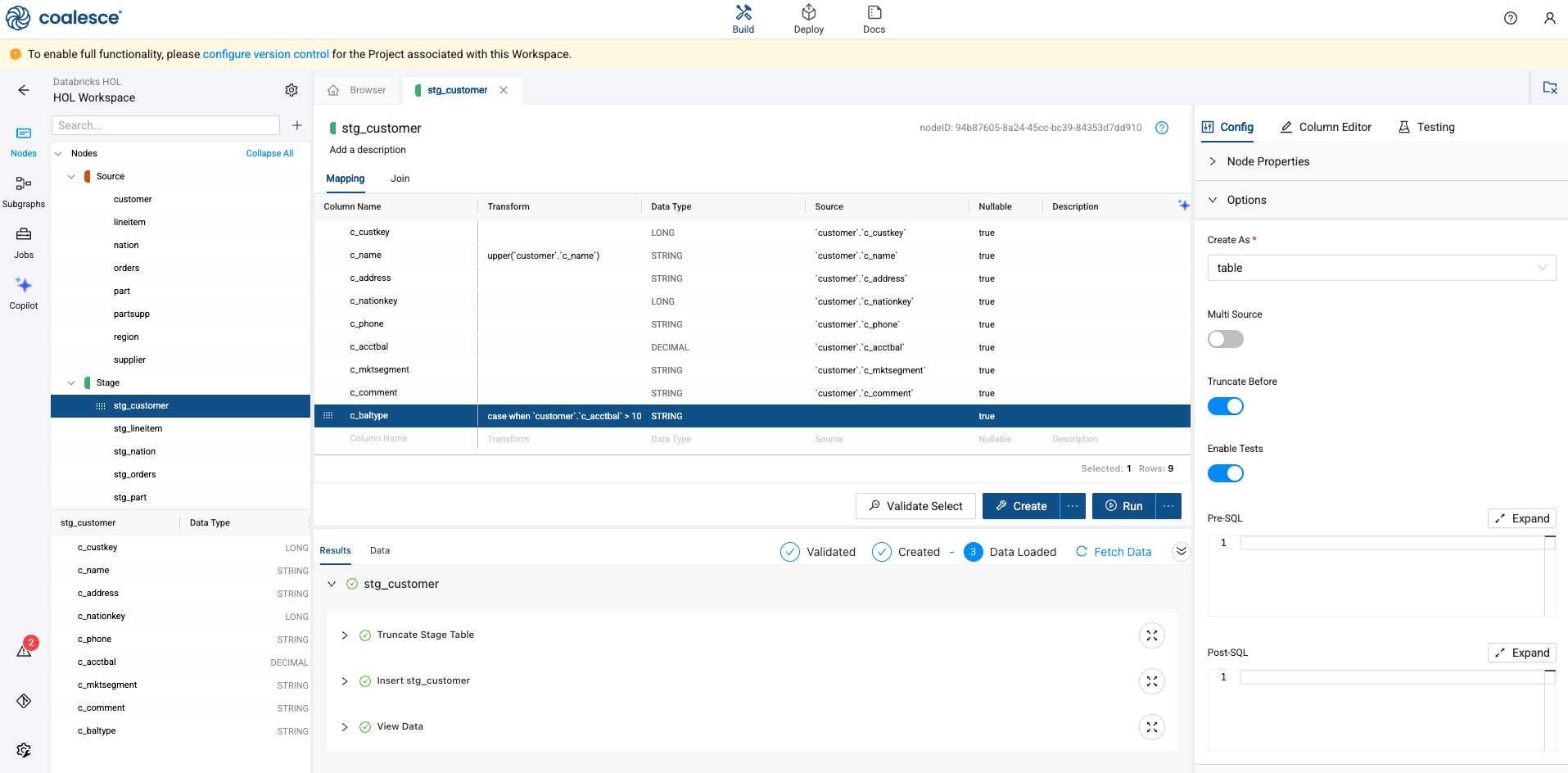
4. Double click on the stg_customer node. This will open the node editor.

   

5. There are three components to the node editor. We will be using all three throughout this lab, so let’s get you familiar. The first is the mapping grid, where we can view our columns, build transformations, supply documentation, and view other metadata.

   

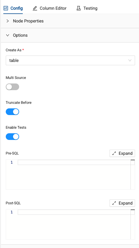
6. Next, to the left of your screen are the configuration options for the node. These options are standardized based on the definition provided when creating the node.

   

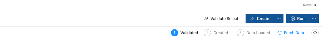
7. Finally, at the bottom of your screen are the Create and Run buttons. Selecting these buttons will execute the DDL and DML respectively for each node.

   

Applying Single Column Transformations

1. Let’s explore how to apply SQL transformations to columns in the mapping grid.

2. Double click into the Transform column of the mapping grid next to the c_name column. This will open a SQL editor for this column. Let’s apply a simple UPPER function to this column.

   UPPER(`customer`.`c_name`)

   

3. Next, let’s add a new column to our table. Double click on the grey “column name” denotation at the bottom of the mapping grid. This will allow you to add a new column by naming it. In this case, let’s call the column c_baltype.

   

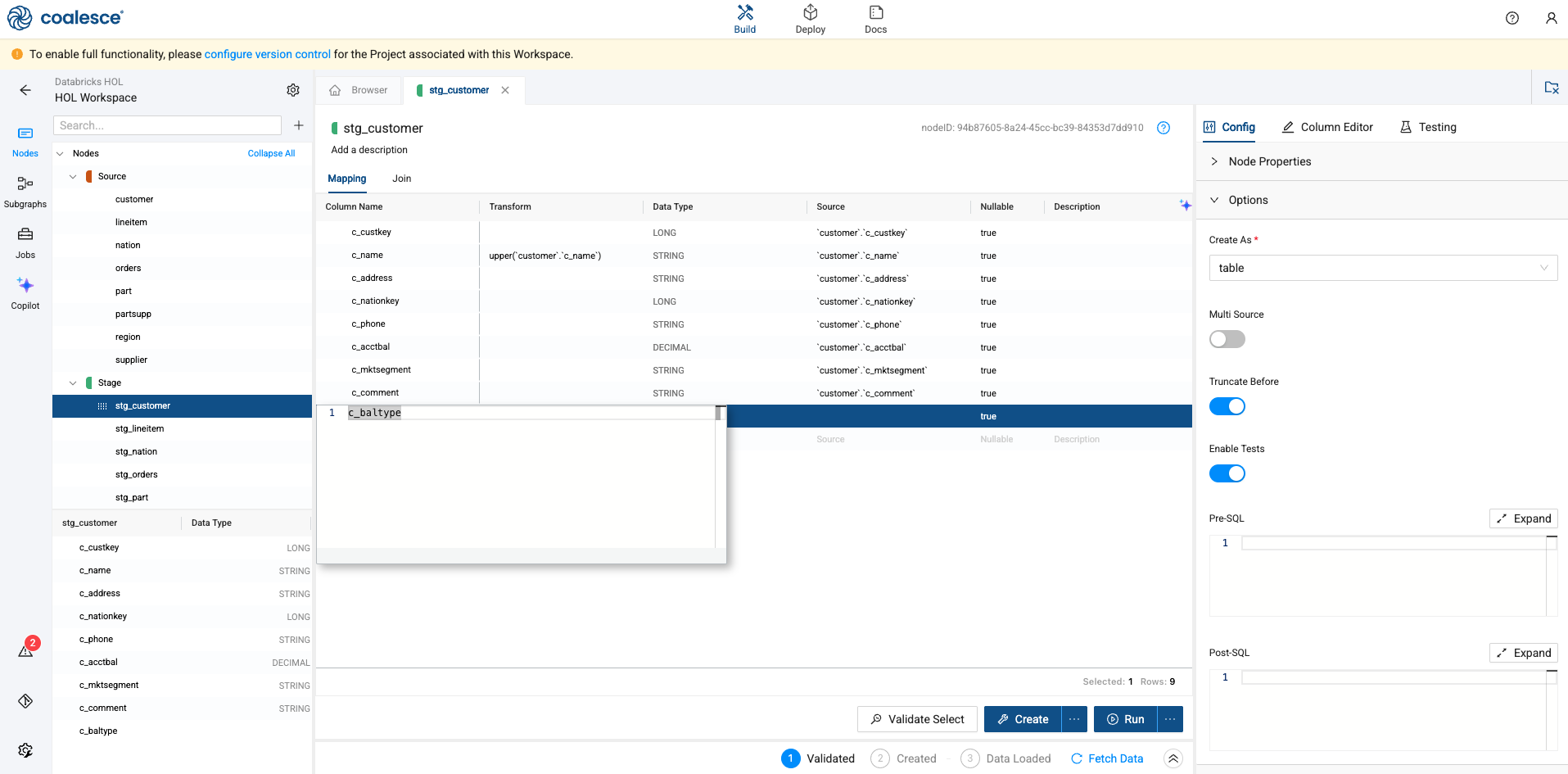
4. When adding a new column, you also need to provide the data type of the column. In this case, we’ll be denoting what type of balance each customer has, so we’ll be using a STRING data type.

   

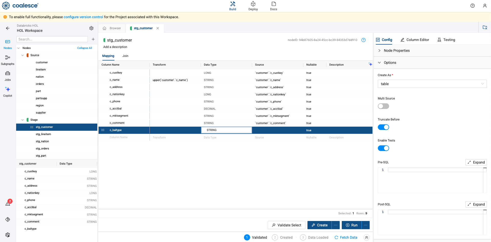
5. Next, we’ll provide CASE WHEN logic to determine what type of balance each customer has. Again, double click into the Transform column of the mapping grid, next to the c_baltype column to open the SQL editor. Supply the following SQL statement

   case when `customer`.`c_acctbal` > 10 then ‘Large’ else ‘Small’ end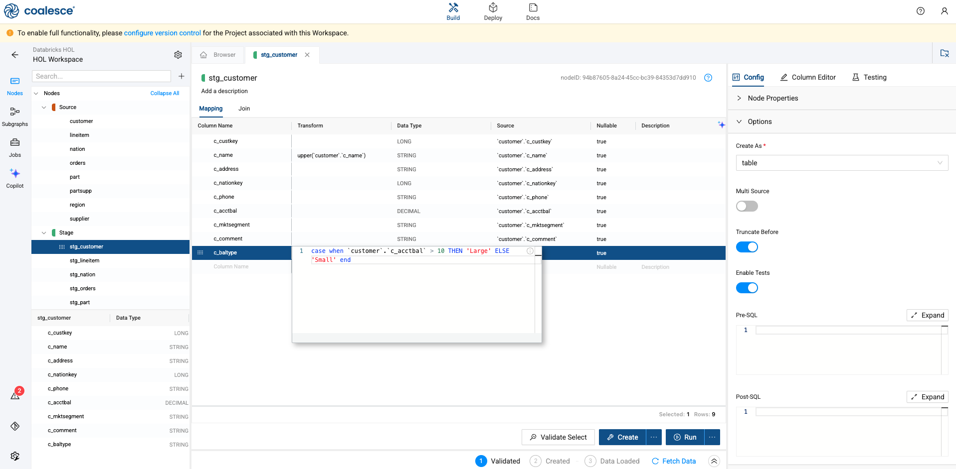

   

6. Once complete, select the blue Create button at the bottom of the screen. This will execute the DDL for the node.

   

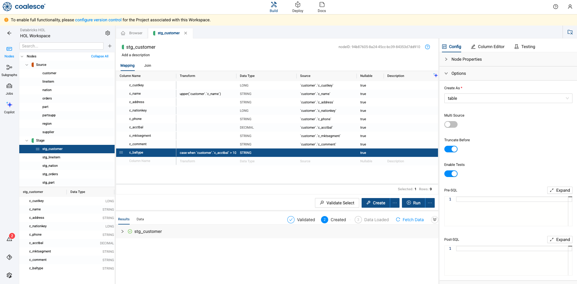
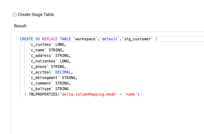
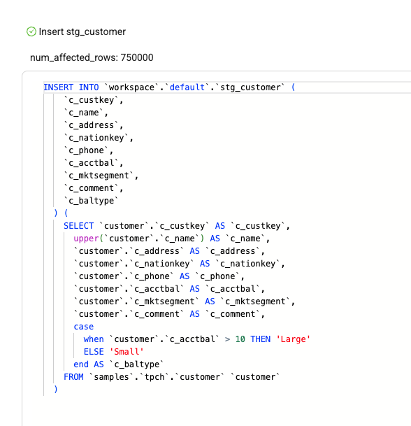
7. Coalesce allows you to view the SQL of each execution at any time. In this case, we can view the exact DDL that was written on your behalf.

   

8. Now that the table is created, select the blue Run button to execute the DML of the table, to populate it with data.

   

9. Coalesce will take into account all of the configuration options and SQL transformations you as a user have provided, and apply them to the DML. In this case, we can view the UPPER and CASE WHEN transformations we applied.

   

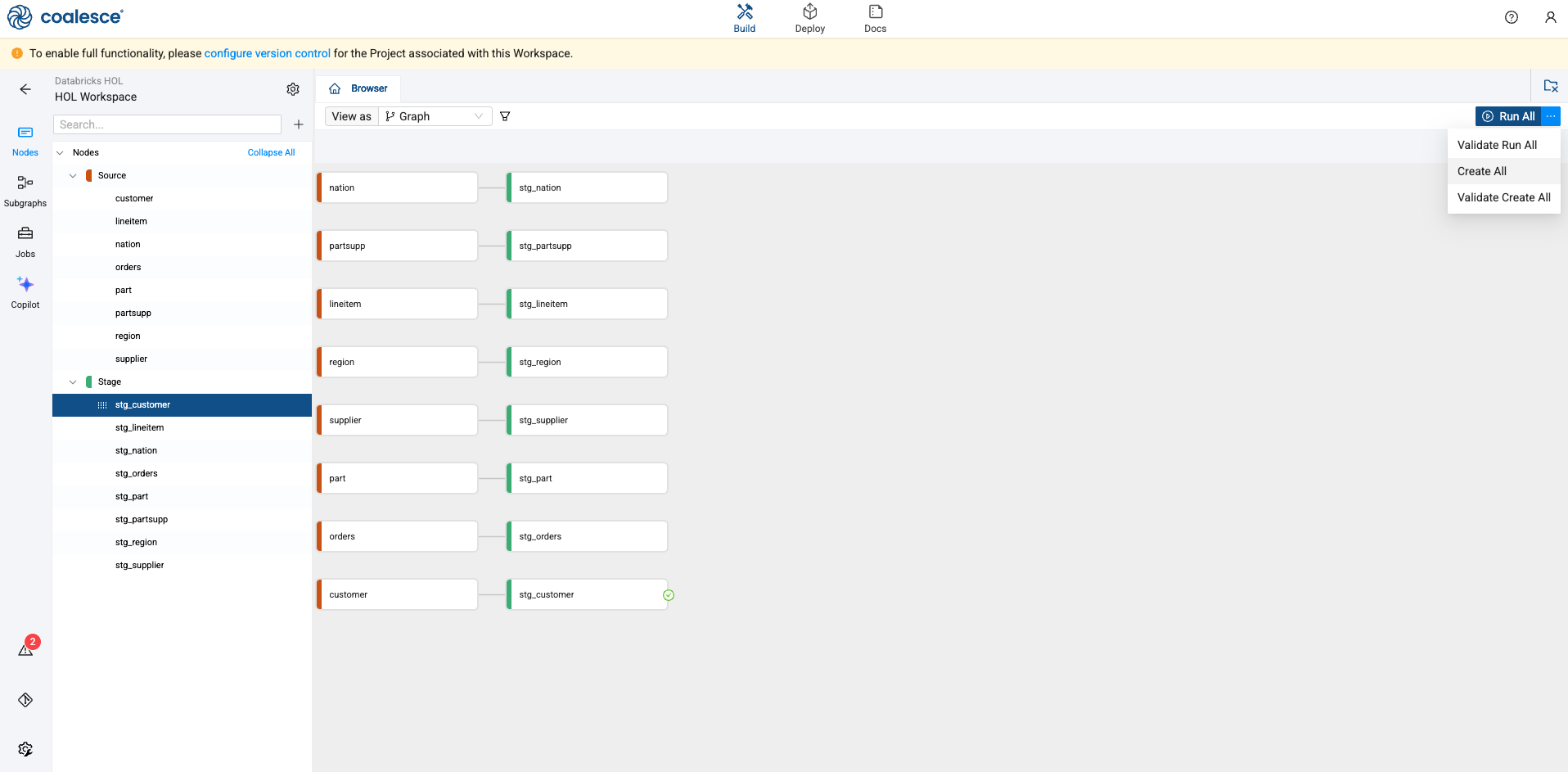
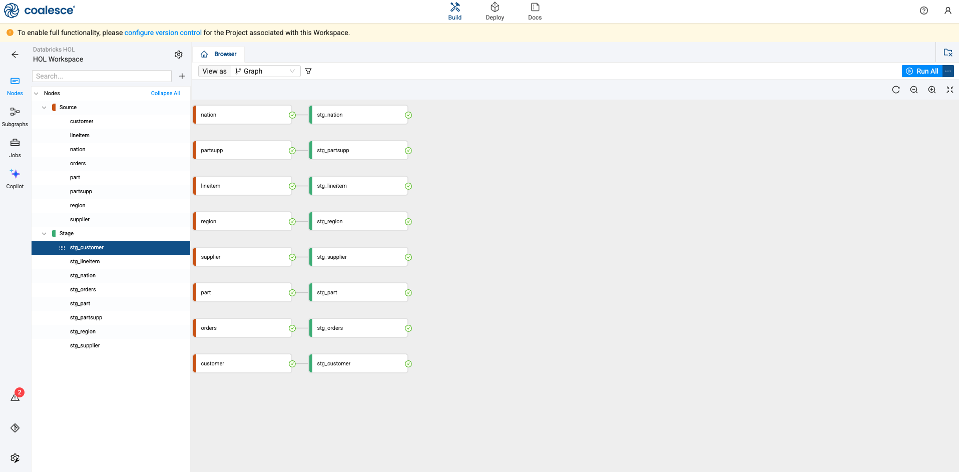
10. Navigate back to the Browser in Coalesce. In the upper right corner of the screen, there is a blue Run All button. Next to it is an ellipsis. Select the ellipsis and choose, Create All. This will execute the DDL for all of the objects in the current pipeline.

    

11. Once complete, select the Run All button to populate all of the tables with data.

    

Joining Nodes

Let’s now join your STG_ORDERS data with your STG_LINEITEM data.

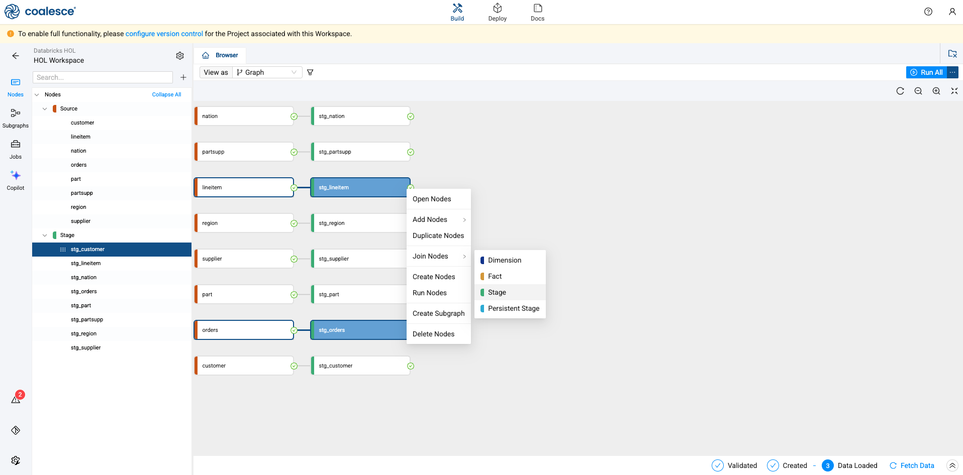
1. Using the shift key on your keyboard, select the stg_orders and stg_lineitem nodes at the same time. Right click on either node and select Join Nodes -> Stage

   

2. Coalesce will drop you inside of the node. Select the pencil icon in the upper left corner of the screen and rename the node to stg_order_master.

   

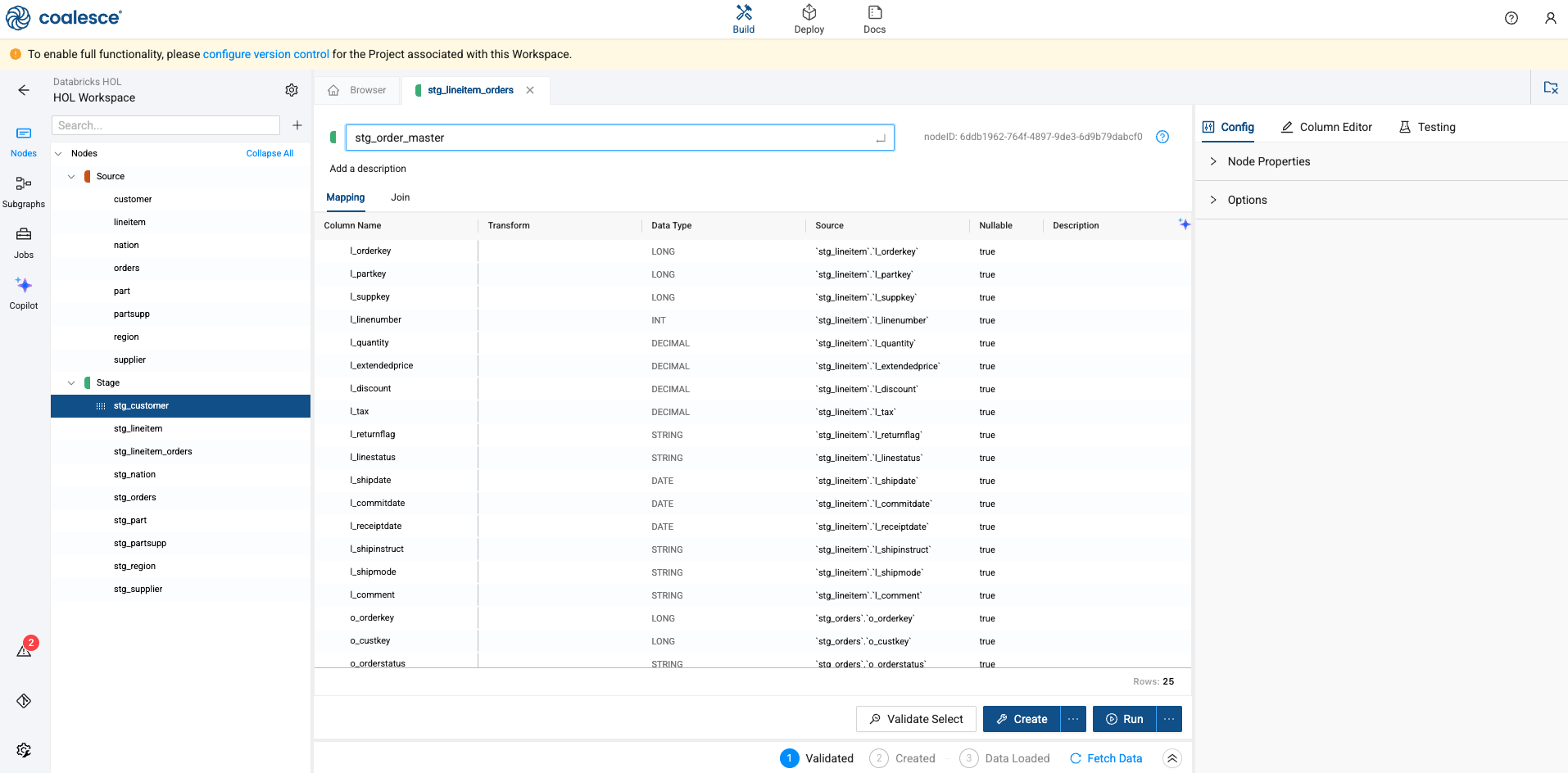
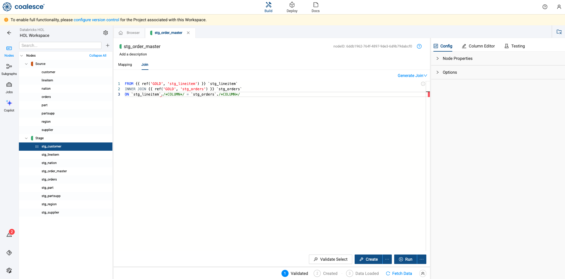
3. Now, select the Join tab of your stG_order_master node in the Node Editor. This is where you can define the logic to join data from multiple nodes, with the help of a generated Join statement.

   

4. Add column relationships in the last line of the existing Join statement using the bolded code below:

   FROM {{ ref('GOLD', 'stg_lineitem') }} `stg_lineitem`
   INNER JOIN {{ ref('GOLD', 'stg_orders') }} `stg_orders`
   ON `stg_lineitem`.`l_orderkey` = `stg_orders`.`o_orderkey`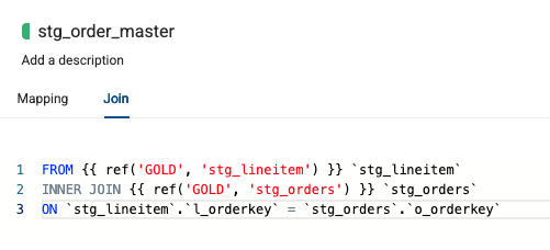

   

5. Select the Create and Run buttons to build the table in Databricks and populate it with data.

6. Let’s perform this same process again with the stg_partsupp and stg_part nodes. Again, hold down the shift key and select both nodes, right click on either node, and select Join Nodes -> Stage.

   

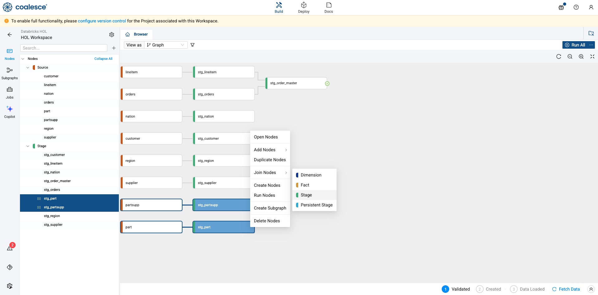
7. Rename the table to stg_part_master.

   

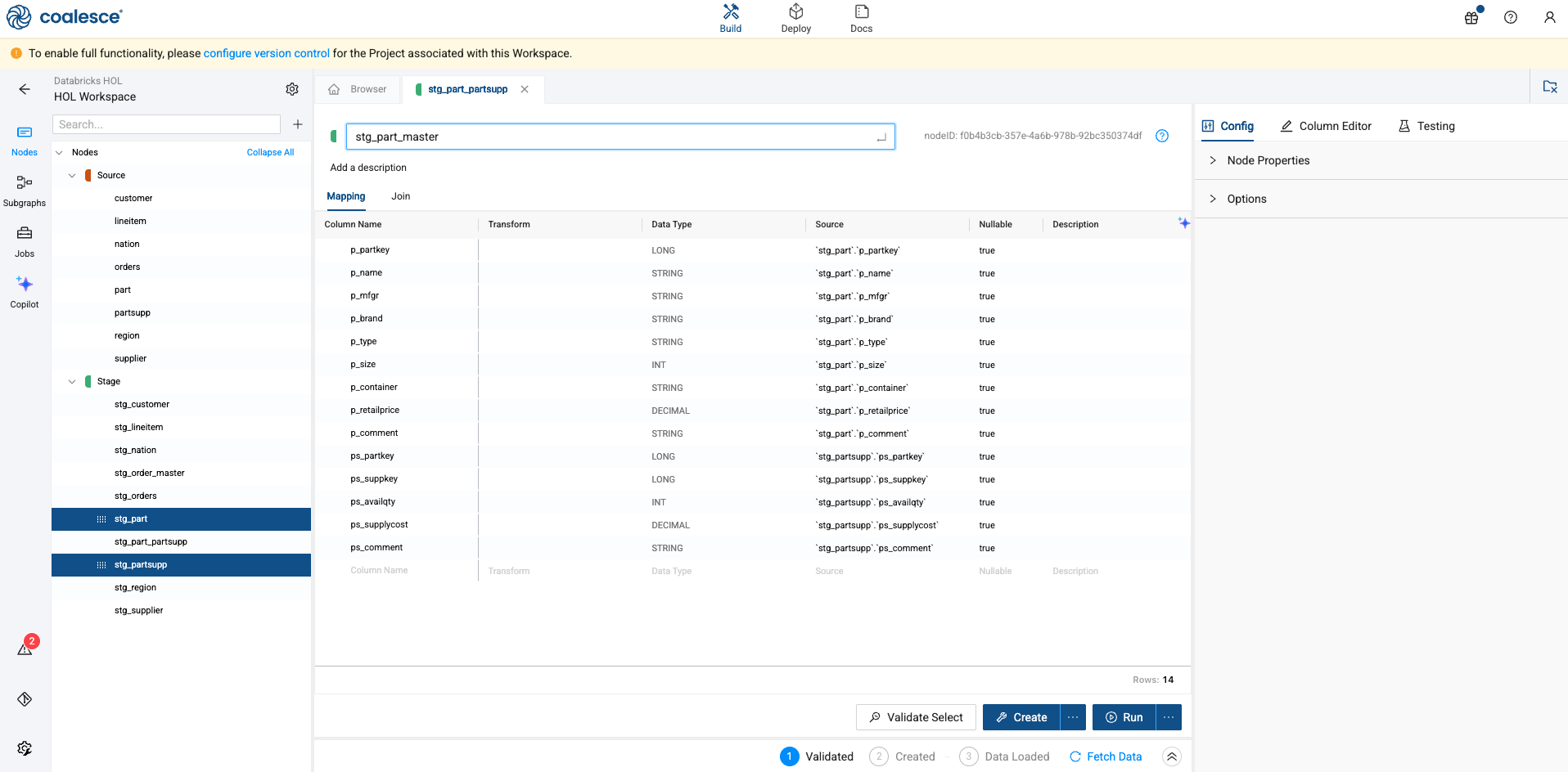
8. Navigate to the join tab and the following join condition:

   FROM {{ ref('GOLD', 'stg_part') }} `stg_part`
   INNER JOIN {{ ref('GOLD', 'stg_partsupp') }} `stg_partsupp`
   ON `stg_part`.`p_partkey` = `stg_partsupp`.`ps_partkey`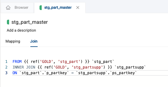

   

9. Create and Run the node to build the table in Databricks and populate it with data. Now you have two joined tables that now exist in your Databricks account.

Creating Dimension Nodes

Now let’s experiment with creating Dimension nodes. These nodes are generally descriptive in nature and can be used to track particular aspects of data over time (such as time or location). Coalesce currently supports Type 1 and Type 2 slowly changing dimensions, which we will explore in this section.

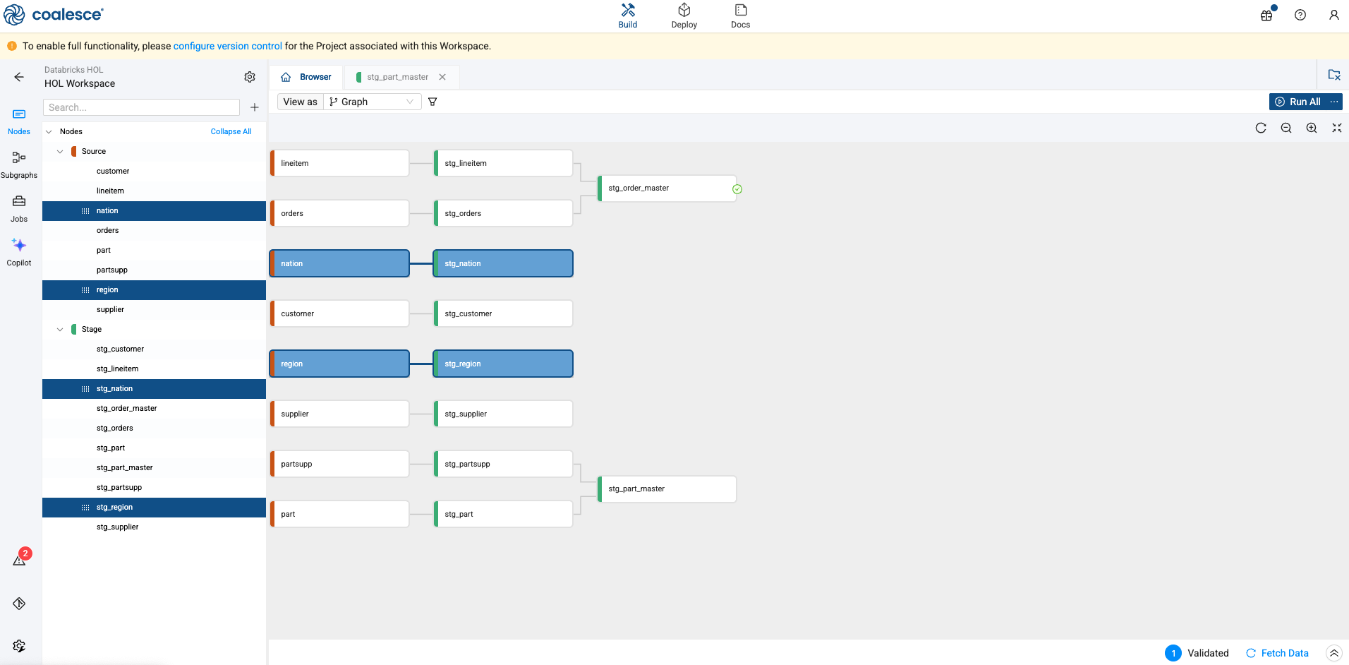
1. First, let’s remove any nodes we no longer need. Let’s remove the nation, stg_nation, region, and stg_region nodes by holding down the shift key and selecting each node. Right click on any of the highlighted nodes and select Delete Nodes.

   

2. With the nodes we care about remaining, again, holding down the shift key, select the stg_customer and stg_supplier nodes, right click on either node, and select Add Nodes -> Dimension.

   

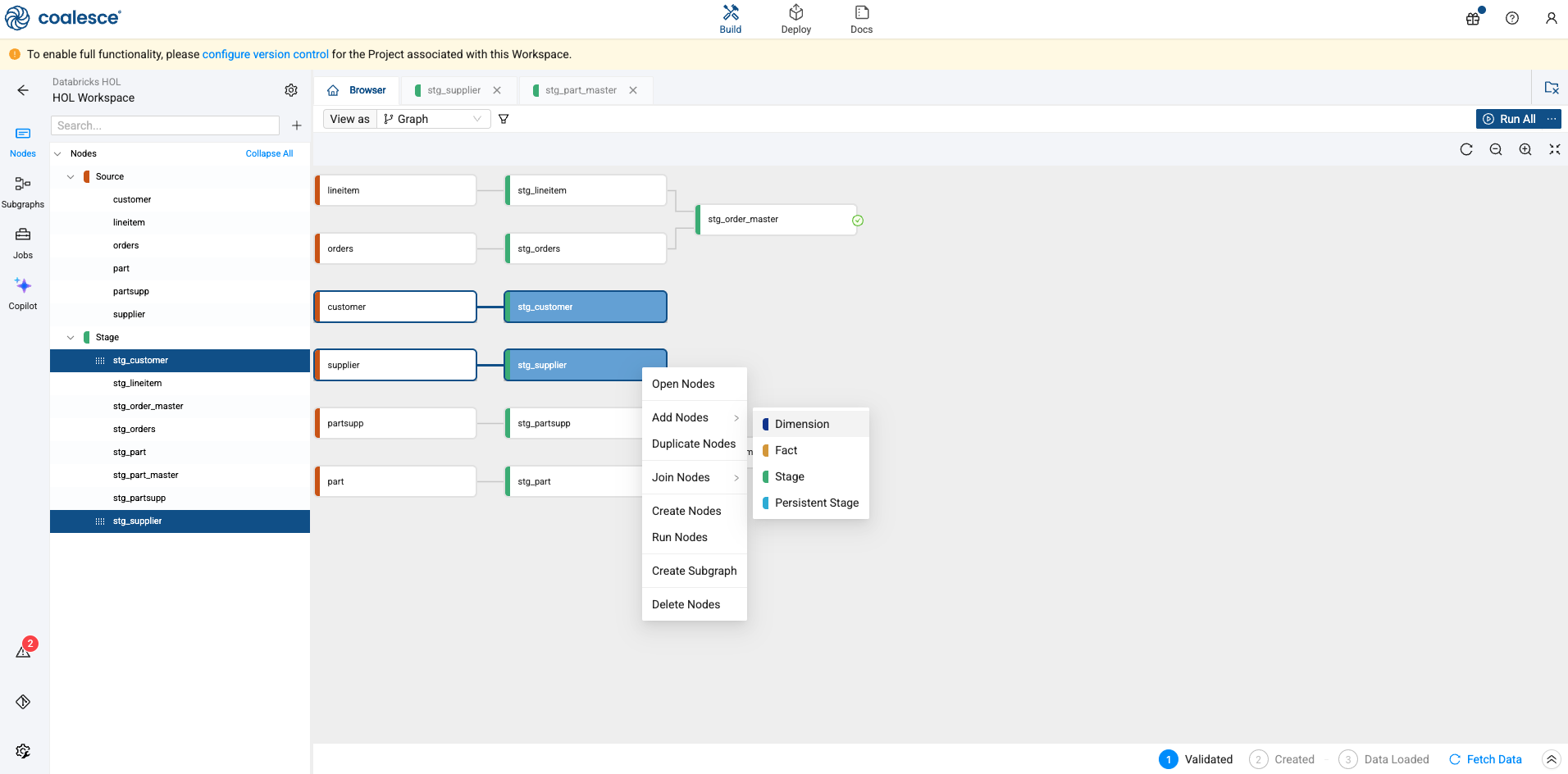
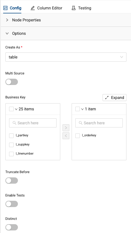
3. This will create two dimension nodes that will be ready to configure. Double click in the dim_customer node.

   

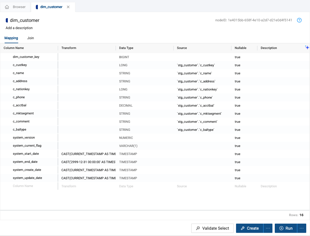
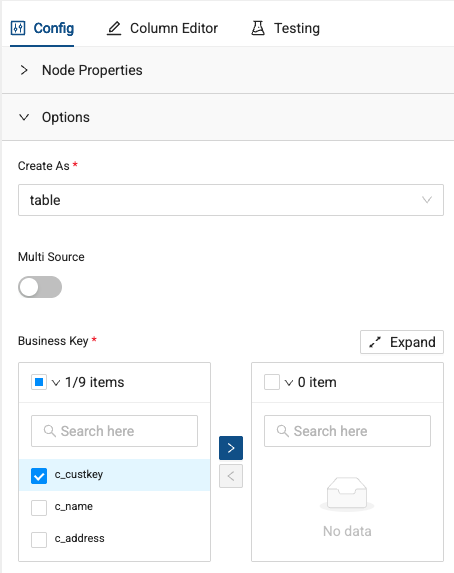
4. The node will look a little different than the stage nodes we’ve been working with. Specifically, within the configuration options, we can specify a business key, as well as change tracking columns for type two slowly changing dimensions. Select c_custkey as the business key for the node.

   

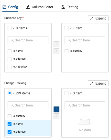
5. Let’s also track changes to columns on this table using the change tracking columns. Select the c_name and c_address columns as the columns we want to track changes on.

   

6. Click Create and Run the dim_customer node. After it is done running, you can view the best practice SQL that Coalesce generated to support type 2 SCDs.

   

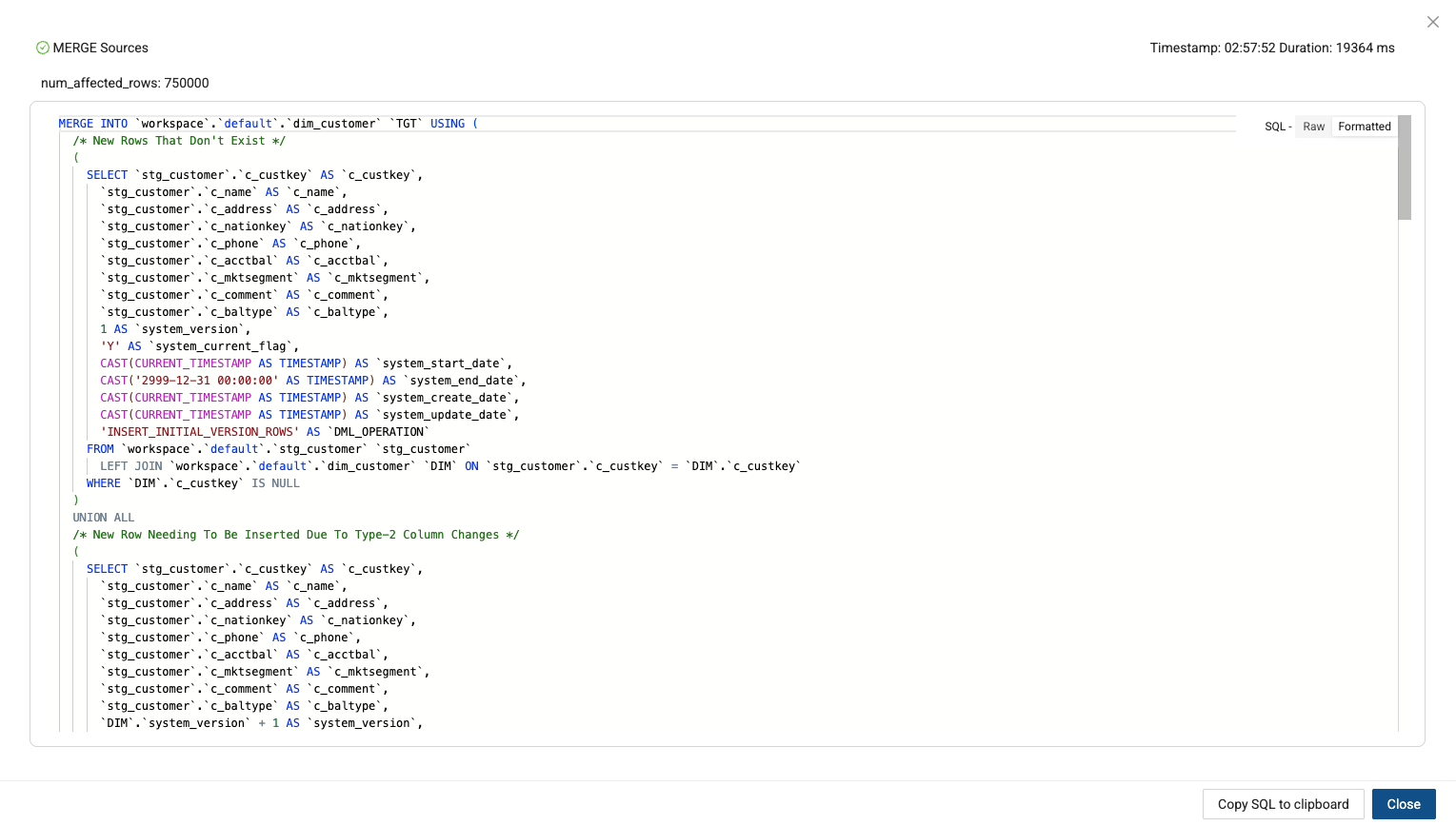
7. Let’s apply this same process to the dim_supplier node.

   

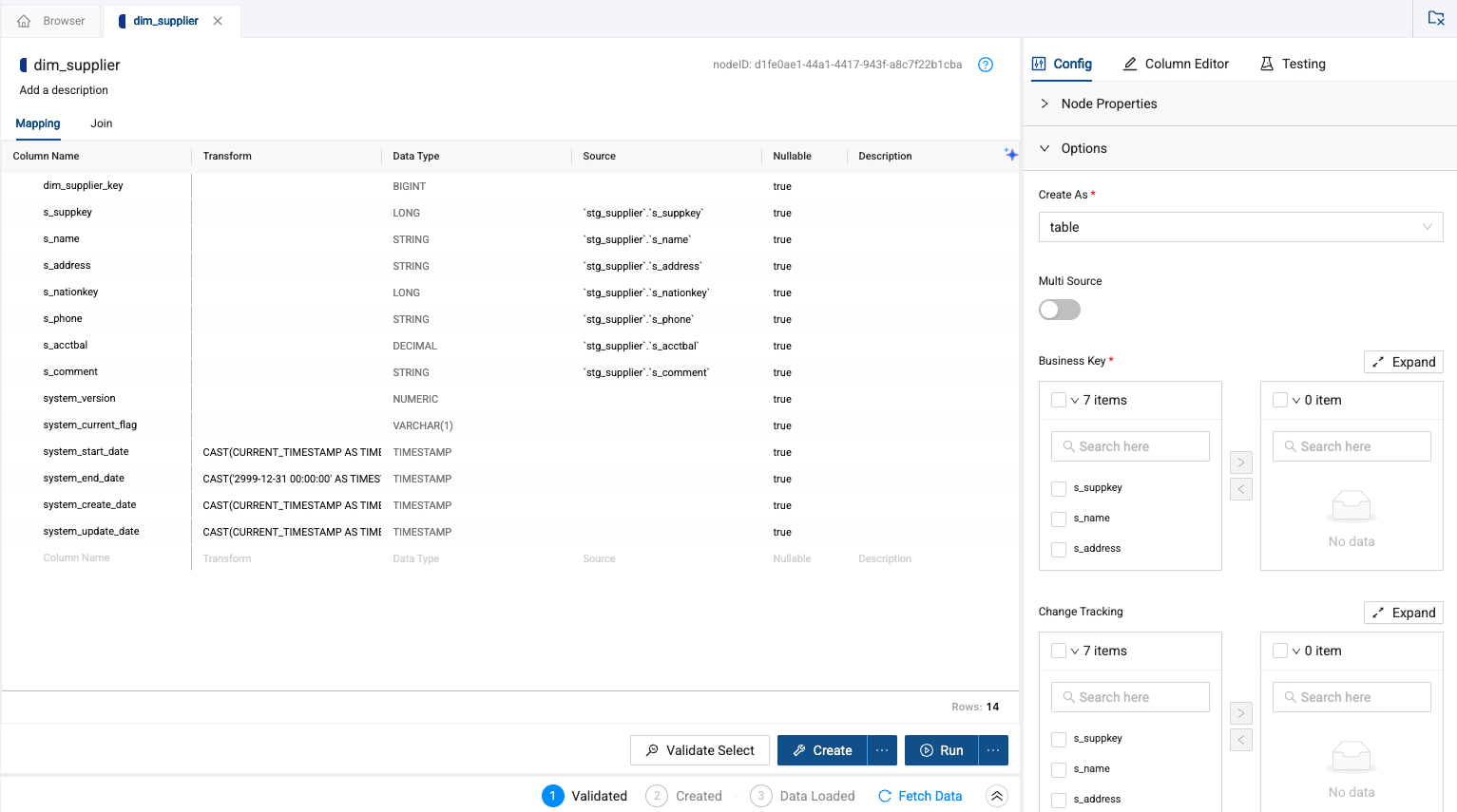
8. Pass the s_suppkey column through as the business key

   

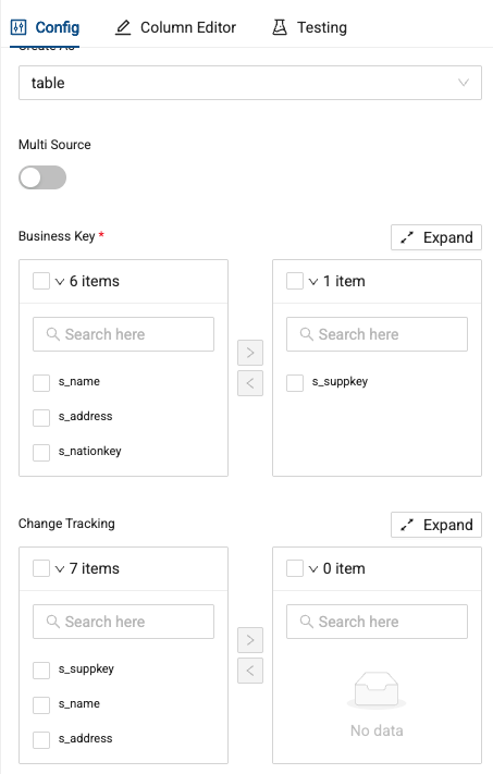
9. This time, we won’t track any changes, so you can just Create and Run the node.

Creating Fact Nodes

Coalesce supports Fact nodes out of the box, which allow you to easily denote tables that are storing fact or measure level data. Let’s learn how to add a fact node.

1. Select and right click on the stg_order_master table. Select Add Node -> Fact

   

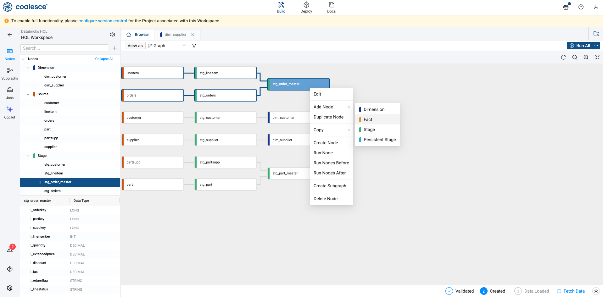
2. You’ll be dropped inside the Fact node. Within the configuration settings, you can select a business key. This is valuable because Coalesce can use this information to infer join conditions when nodes are joined together. In this case, use the l_orderkey as the business key.

   

3. Create and Run the node and view your graph

   

Adding a View for Reporting

Coalesce supports views for various use cases within data pipelines. In order to use view nodes, you need to turn them on first.

1. Navigate to the build settings in the lower left corner of the screen and select the gear icon.

   

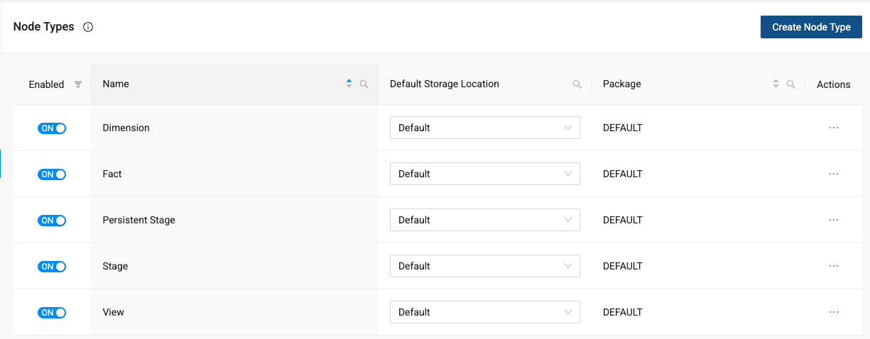
2. Navigate to Node Types to view all of the nodes available in your workspace. You can see the View is toggled to off.

   

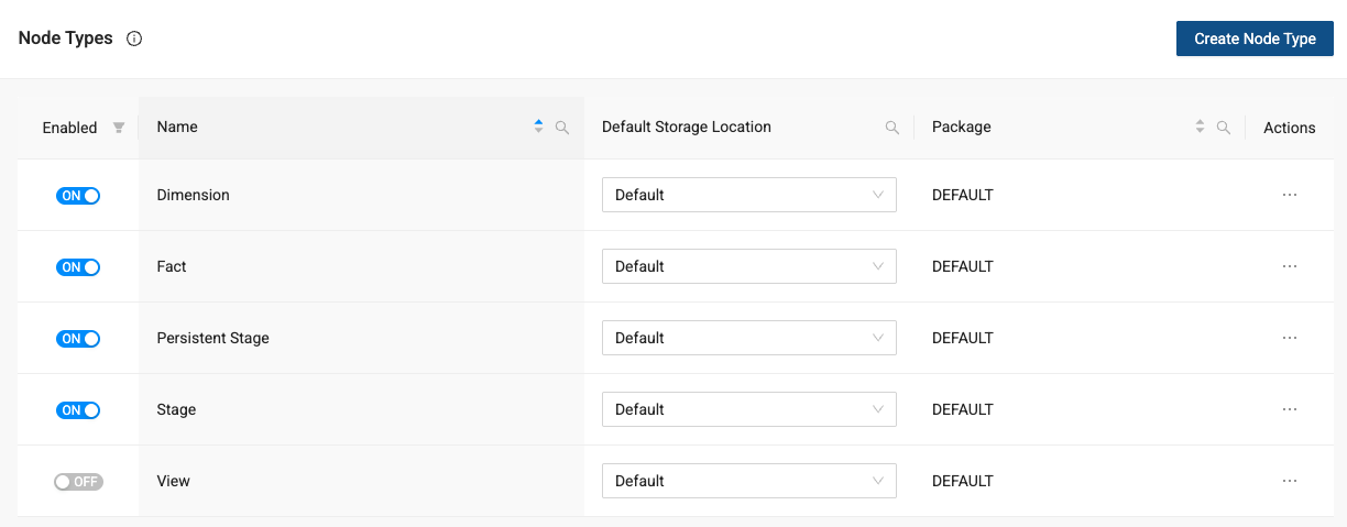
3. To turn a view on, select the toggle to turn it on.

   

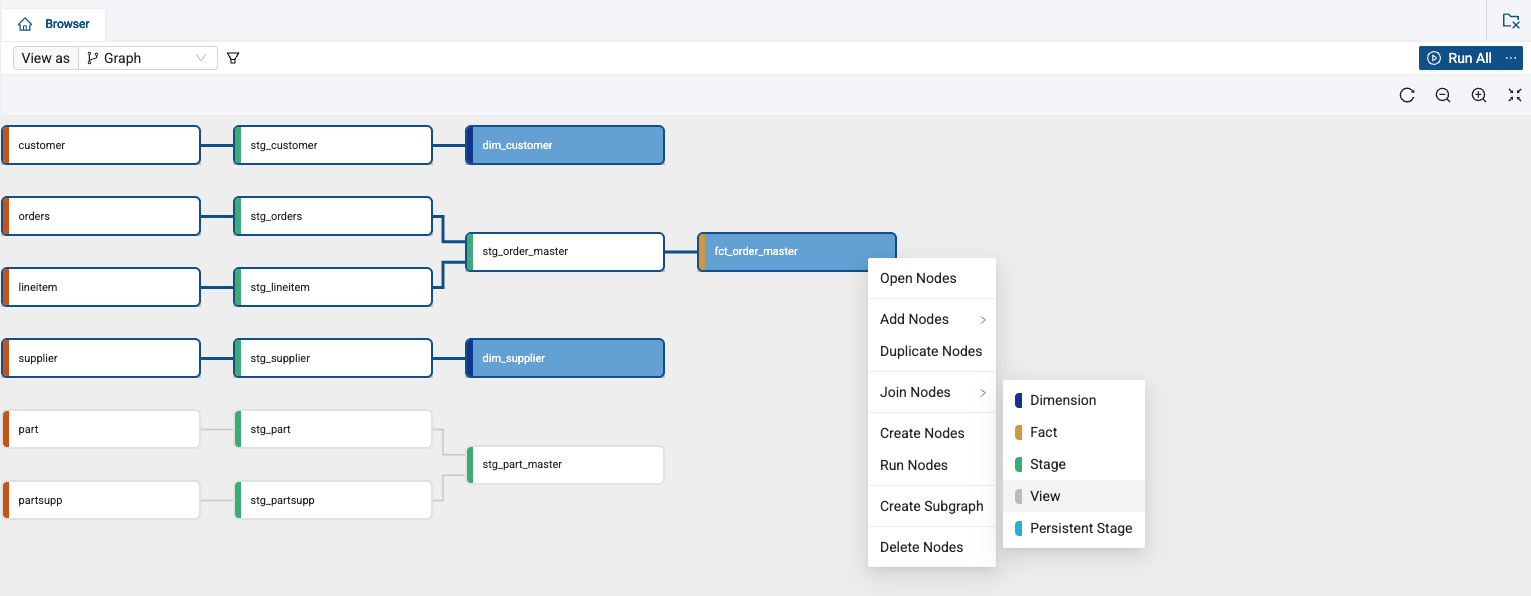
4. Now, navigate back to the Browser and we’ll join a small star schema together into a view. By holding down the shift key, select the fct_order_master, dim_customer, and dim_supplier nodes, right click on either of them and select Join Nodes -> View.

   

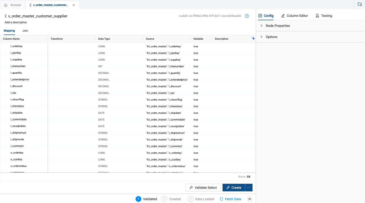
5. Inside the node, you’ll see all of the columns from all three tables.

   

6. Let’s configure the join first. Navigate to the join tab to configure the join. Supply the following join condition below:

   FROM {{ ref('GOLD', 'fct_order_master') }} `fct_order_master`
   LEFT JOIN {{ ref('GOLD', 'dim_customer') }} `dim_customer`
   ON `fct_order_master`.`o_custkey` = `dim_customer`.`c_custkey`
   LEFT JOIN {{ ref('GOLD', 'dim_supplier') }} `dim_supplier`
   ON `fct_order_master`.`l_suppkey` = `dim_supplier`.`s_suppkey`

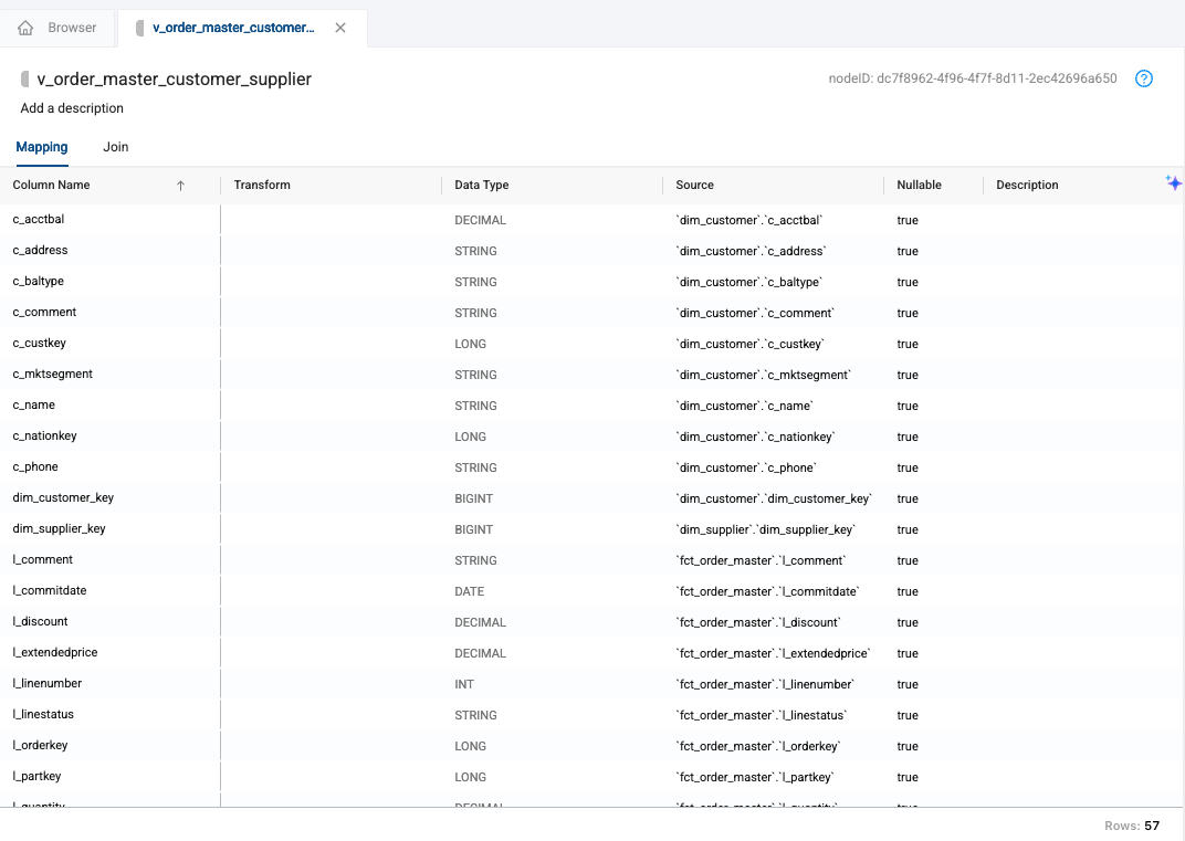
7. Now navigate back to the mapping grid. We need to remove columns that have the same name, plus get rid of columns we no longer need. Select the Column Name header on the mapping grid to alphanumerical sort your columns

   

8. Scroll down to the bottom of the mapping grid to view all of the system columns available. Select the very first system column listed, hold down the shift key, and select the last system column selected. Then, right click on any of the highlighted columns and select Delete Columns.

   

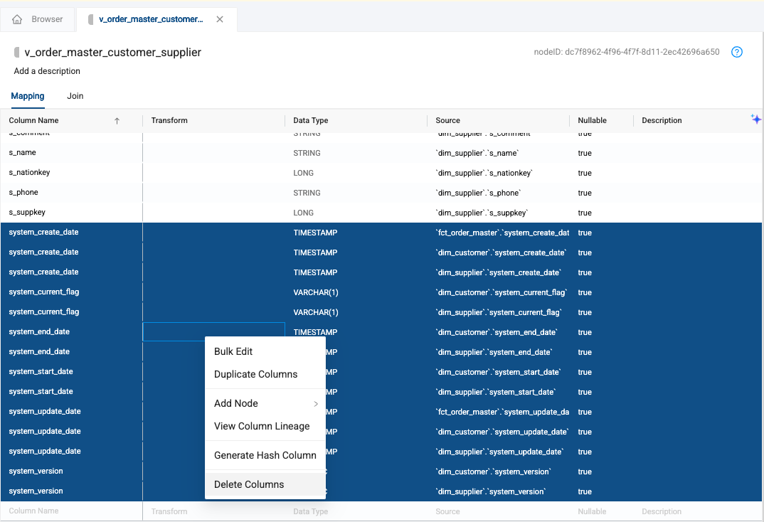
9. You will need to confirm you want to delete these columns. Select Delete.

   

10. Create the view! You will notice there is no run button, because views are just stored as queries, they don’t actually store data.

Bulk Editing Columns, Tests, and Propagation

With your pipeline built, you can add tests to your nodes to ensure your data quality is intact. Additionally, once done, as new columns are added to your pipeline, propagating those changes easily can be incredibly important. Finally, it can be tedious to manually write and update data transformations for each individual column. With Coalesce, you can bulk edit columns quickly and easily. That’s what we’ll learn about in this last section.

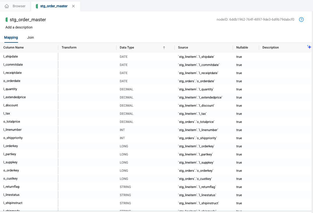
1. In the Browser, double click on the stg_order_master node to open it.

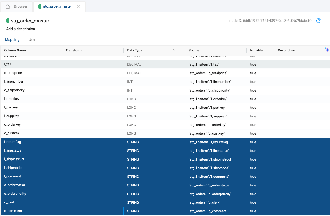
2. Select the Data Type Column header in the mapping grid to sort the columns in alphanumerical order by data type.

   

3. All of the STRING data types will be at the bottom of your screen. By holding down the shift key, we can select the first column containing a STRING data type, and then the last column containing a STRING data type.

   

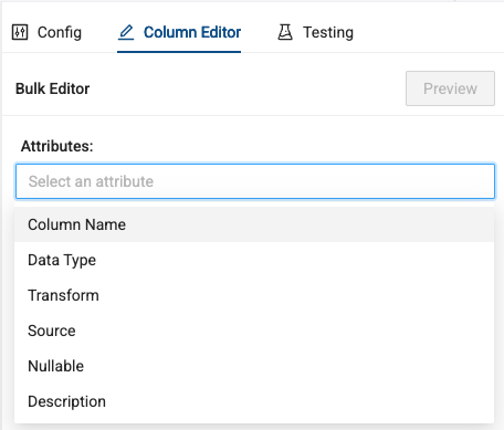
4. Right click on any of the highlighted columns and select Bulk Edit

   

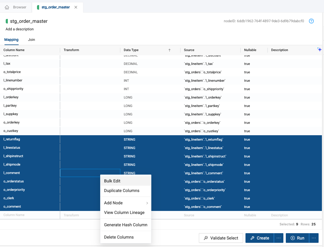
5. Within the Column Editor on the right side of the screen, select the attribute you want to update - in this case, Transform.

   

6. A SQL editor will open where you can write the SQL statement that you want applied to all of the columns highlighted. We’ll use the SQL statement below, to apply lower casing to all of the columns in our columns.

   lower({{SRC}})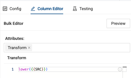

   

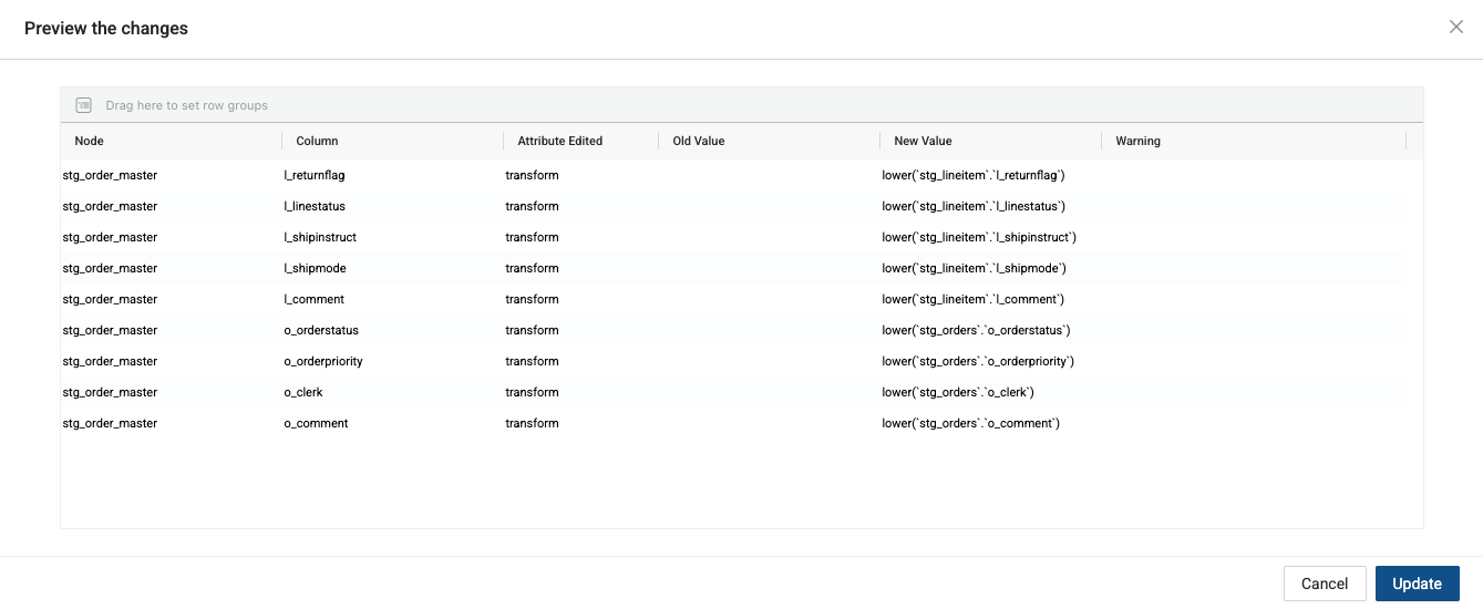
7. Select the Preview button to view your changes and select Update to persist the changes to your columns.

   

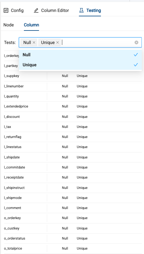
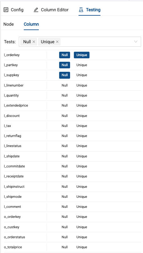
8. Next, in the Testing tab in the upper right corner of the node, you can write your own SQL based tests, or use out of the box, null or unique column tests. Navigate to the Column section of the Testing tab.

   

9. Select both Null and Unique as values you want to test for.

   

10. Next, select Null for each of the following three keys:

    • l_orderkey
    • l_partkey
    • l_suppkey

11. These tests check to ensure that no null values are contained within these columns. You should also select the Unique test for the l_orderkey column.

    

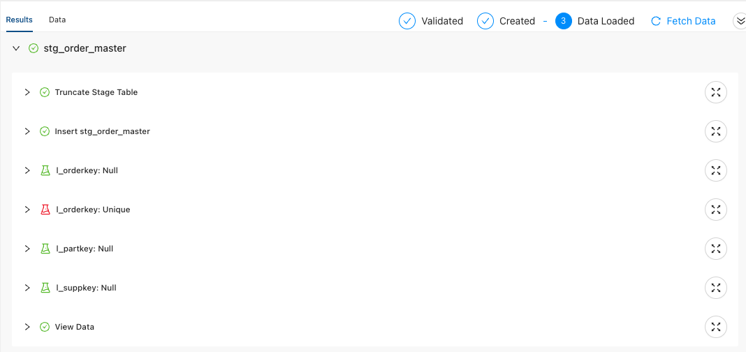
12. When you run the node, you’ll be able to see each execution step. Notice that the Unique test on l_orderkey failed. This is because for each line item contained in an order, the order key will be listed. This means if there were 5 line items in an order, the order ID will duplicate 5 times.

    

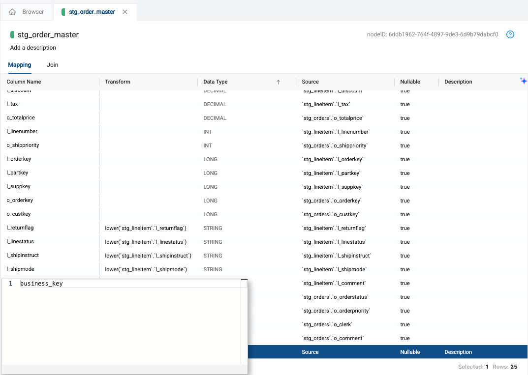
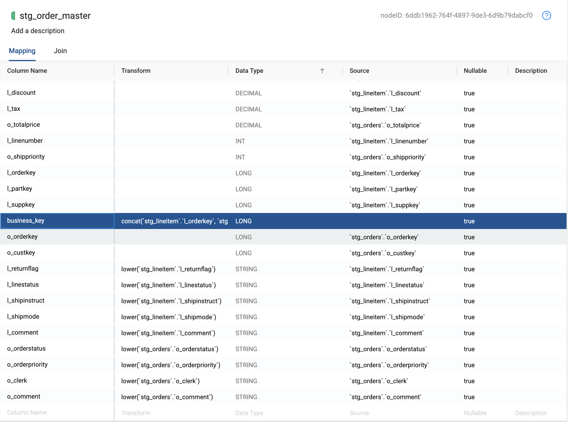
13. To solve this, let’s create a business key that is unique to the table. Create a new column called business_key.

    

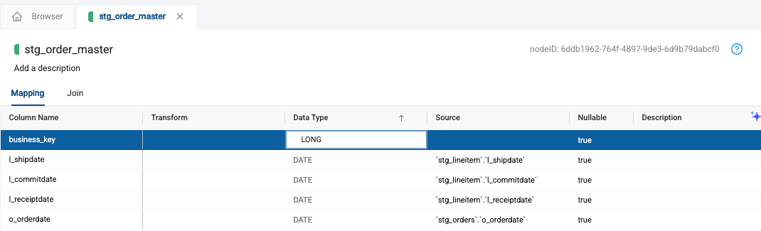
14. Give it a data type of LONG.

    

15. Next, let’s create the unique identifier for the table by providing a transformation that concatenates the l_orderkey and l_linenumber together.

    concat(`stg_lineitem`.`l_orderkey`, `stg_lineitem`.`l_linenumber`)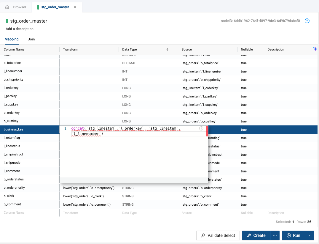

    

16. Create and Run the node to make the changes.

17. Drag the business_key node to the middle of the mapping grid - this allows us to arrange columns in a more helpful order.

    

18. Back in the Testing tab, deselect the Unique test from l_orderkey and select the Unique test for the new business_key column.

    

19. Now, rerun the node and ensure all the tests pass. Congratulations! You’ve successfully, built, transformed, and tested your data.

Conclusion and Next Steps

Congratulations on completing this entry-level lab exercise! You've mastered the basics of Coalesce and are now equipped to venture into our more advanced features. Be sure to reference this exercise if you ever need a refresher.

We encourage you to continue working with Coalesce by using it with your own data and use cases and by using some of the more advanced capabilities not covered in this lab.

What we’ve covered

• How to navigate the Coalesce interface
• How to add data sources to your graph
• How to prepare your data for transformations with Stage nodes
• How to join tables
• How to apply transformations to individual and multiple columns at once
• How to build out Dimension and Fact nodes
• How make and propagate changes to your data across pipelines

Continue with your free trial by loading your own sample or production data and exploring more of Coalesce’s capabilities with our and .

Reach out to our sales team at coalesce.io